Week 7 - Simulation of a 1D Super-sonic nozzle flow simulation using Macormack Method
Approach for Solving 1D Super-sonic nozzle flow simulation via MacCormack Method
- Solving the 1D nozzle flow problem in two approaches: Non-Conservative approach and Conservative approach using McCormack method.
- Conservative approach, the assumed control volume is fixed in position and in Non-conservative approach, the control volume is moving.
- Convergence is checked using error and tolerance method. Also, time stepping until 1400 time steps is done for comparison with the reference book: John.D.Anderson
1.GOVERNING EQUATIONS
a) NON CONSERVATIVE APPROACH:
CONTINUITY EQN
∂ρ/∂t = -ρ*(∂v/∂x) – ρv * (∂(lnA)/∂x) – v*(∂ρ/∂x)
MOMENTUM EQN
∂v/∂t = -v*(∂v/∂x) – (1/γ)*(∂T/∂x + (T/ρ)∂ρ/∂x)
ENERGY EQN
∂T/∂t = -v*(∂T/∂x) - (γ-1)*T*(∂v/∂x + v*∂(lnA)/∂x)
b) CONSERVATIVE APPROACH:
CONTINUITY EQN
∂(ρA)/∂t + ∂(ρ.A.v)/∂x = 0
MOMENTUM EQN
∂(ρAv)/∂t + (∂(ρAv2)+(1/γ)⋅pA)/∂x=(1/γ)*p*(∂A/∂x)
ENERGY EQN
∂ ρA(e/(γ-1)+(γ/2)V2)/∂t + ∂ρ((e/(γ-1)+(γ/2)V2)VA + pAV)/∂x = 0
*Referring to the (Pg339) excerpt by J D Anderson in his book on CFD, when the governing equations are solved in primitive/conservative form as shown above, some stability issues are encountered and hence the equations are written in 'Pure' form. Let us define the elements of Solution Vector U, Flux Vector F & Source Term J as following:
U1=ρ` A`
U2=ρ` A` V`
U3=ρ` (e`/(γ-1)+(γ/2) V`2)A`
F1=ρ` A` V`
F2=ρ`A`V`2+(1/γ) p`A`
F3= ρ` (e`/(γ-1)+(γ/2) V`2)A`V`+ρ`A`V`
J2=(1/γ)P`(∂A`/∂x`)
Substituting the above elements:
∂U1/∂t`=-∂F1/∂x`
∂U2/∂t`=-∂F2/∂x`+J2
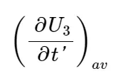
∂U3/∂t`=-∂F3/∂x`
Governing equations are then Discretized using the MacCormack's method
Step1: Predictor step
To start the calculation, we use the initial conditions for U1, U2, and U3 to calculate the initial values of F1, F2, and F3 and and we use these values to calculate the values of U1,U2 and U3 in the next time step . We Calculate the time derivatives by using forward difference for space(dx) terms and these time derivatives are used to calculate the predicted values of U1 ,U2 and U3.
Step2: Corrector Step
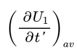
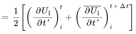
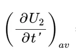
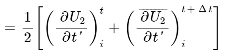
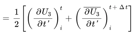
Now using the predicted values we calculate the new flux terms and source terms .Then we calculate the time derivative terms by using backward difference.Then we calculate the average values of time derivatives of predictor and corrector steps .
Step3: Calculation for Next time Step
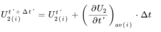
Then we calculate the corrected values of U1,U2,U3 by using average values of time derivative.This is done at every node except the boundary nodes since we calculate them by using boundary conditions.These steps are to be repeated until steady state is obtained.


2.INITIAL AND BOUNDARY CONDITIONS:
a) NON CONSERVATIVE FORM
- At inlet boundary(subsonic inflow),
Here 'n' => nth Node
v(1)=2⋅v(2)-v(3); -- through interpolation
ρ(1)=1
t(1)=1
- At outlet boundary(supersonic outflow boundary at point N),
All boundary conditions at outlet are obtained through Extrapolation.
v(n) =2⋅v(n-1) - v(n-2)
ρ(n) =2⋅ρ(n-1) - ρ (n-2)
t(n) =2⋅t(n-1) - t (n-2)
- INITIAL CONDITIONS,
For 0≤ x ≤ 3;
ρ=1-0.3146x
t=1-0.2314x
v=(0.1+1.09x) t0.5
a=1+2.2(x-1.5)2
b) CONSERVATIVE FORM:
- At inlet boundary,
Here 'n' =>nth Node.
ρ(1)=1
U1=ρ(1)⋅a(1)
v(1)=U2(1)/U1(1)
t(1)=1
U3(1)=U1(1) (t(1/γ-1)+γ*0.5*v(1)2)
- At outlet boundary, (Using extrapolation techniques)
U1(N) =2⋅U1(N-1) -U1 (N-2)
U2(N) =2⋅U2(N-1) -U2 (N-2)
U3(N) =2⋅U(N-1) -U3 (N-2)
- INITIAL CONDITIONS:
- When 0≤ x`≤0.5 ; ρ`= 1.0 & T`= 1.0
- When 0.5≤ x`≤1.5 ; ρ`= 1-0.366(x`-0.5) & t`=1-0.167(x`-0.5)
- When 1.5≤ x`≤3.5 ; ρ`= 0.634-0.3879(x`-1.5) & t`=0.833-0.3507(x`-1.5)
3. TIME STEP Calculation(dt)
CFL condition to find the value of 'dt' :
△t = C*△x/ ((T^0.5) + V)
'T' => speed of sound
'V' => local speed of sound.
Δt calculated at all the grid points, i = 1 to i = N, by taking C =0.5, the minimum value is selected.
%Main Code
%Simulation of 1D Supersonic Nozzle Flow using Macromack Method
clear all
close all
clc

% Taking grid points
n =31;
%As 1D it is along x-axis (Nozzle)
x = linspace(0,3,n);
dx = x(2)-x(1);
%Area of Nozzle
A = 1+2.2*(x-1.5).^2;
%gamma
gamma  = 1.4;
%Time steps
nt = 1400;
%Courant Number
C= 0.5;

%Throat Values
throat = ((n-1)/2);

%Non-Conservative Form Function
tic
[V,rho,T,m,M,P,V_t,rho_t,T_t,m_t,M_t,P_t]= non_consv(x,gamma,dx,A,n,nt,C,throat);
non_consv_form = toc;

%Non-Conservative Form Function
tic
[Vc,rhoc,Tc,mc,Mc,Pc,V_tc,rho_tc,T_tc,m_tc,M_tc,P_tc] = consv_func(x,gamma,dx,A,n,nt,C,throat);
consv_form   = toc;

%Plots for Conservative vs Non conservative Form
%Mass Flow rate
figure(3)
subplot(3,2,1)
plot(x,m)
hold on
plot(x,mc,'o')
xlabel('length of  nozzle(x)');
ylabel('Mass flow rate (m)');
title('Mass flow rate Cosnv vs Non-Consv');
grid on

% Variation in non dimensional flow parameters along x-axis
% Mach number
subplot(3,2,2)
plot(x,M);
hold on
plot(x,Mc,'o');
grid on;
xlabel(' length (x)');
ylabel('Mach Number');
legend('Non Conservative Form', 'Conservative Form');
title('Mach Number')

% pressure
subplot(3,2,3)
plot(x,P);
hold on
plot(x,Pc,'o');
grid on;
xlabel('length (x)');
ylabel('Pressure');
legend('Non Conservative Form', 'Conservative Form');
title('pressure Profile')

% Density
subplot(3,2,4)
plot(x,rho);
hold on
plot(x,rhoc,'o');
grid on;
xlabel(' length (x)');
ylabel('Density');
title('Change in density in x-axis')

% Temperature
subplot(3,2,5)
plot(x,T);
hold on
plot(x,Tc,'o');
grid on;
xlabel(' length of Nozzle');
ylabel('Temperature');
title('Change in tempertaure')
% Velocity
subplot(3,2,6)
plot(x,V);
hold on
plot(x,Vc,'o');
grid on;
xlabel('length (x)');
ylabel('Velocity');
title('velocity along x-axis')

% Variation of flow properties at throat.
figure(4)
subplot(4,1,1);
plot(1:nt,rho_tc);
hold on
plot(1:nt,rho_t, 'color', 'r');
grid on
ylabel('Density');
title('density variation at each time step at throat');

subplot(4,1,2);
plot(1:nt,T_tc);
hold on
plot(1:nt,T_t);
grid on
ylabel('Temperature');
title('tempertaure variation at each time step at throat');

subplot(4,1,3);
plot(1:nt,P_tc);
hold on
plot(1:nt,P_t);
grid on
ylabel('Pressure');
title('pressure variation at each time step at throat');


subplot(4,1,4);
plot(1:nt,M_tc);
hold on
plot(1:nt,M_t);
grid on
xlabel('Time step')
ylabel('Mach Number');
title('Mach number variation at each time step at throat');
%Non-Conservative Form Function:
function[V,rho,T,m,M,P,V_t,rho_t,T_t,m_t,M_t,P_t] = non_consv(x,gamma,dx,A,n,nt,C,throat)
%Initial Conditions
rho = 1-0.3146*x;
T = 1-0.2314*x;
V = (0.1+1.09*x).*T.^0.5;
%Time steps calculated using Courant Number For Optimal Value
dt = min(C.*dx./(sqrt(T)+V));
%Outer Time loop
for k = 1:nt
%Copying Values to old
rho_old = rho;
T_old = T;
V_old = V;
%predictor step
for i = 2:n-1
dvdx_predictor = (V(i+1)-V(i))/dx;
dtdx_predictor = (T(i+1)-T(i))/dx;
drhodx_predictor = (rho(i+1)-rho(i))/dx;
dlog_Adx_predictor = (log(A(i+1))-log(A(i)))/dx;
%continuity equation
drhodt_p(i) = -(rho(i)*dvdx_predictor)-(rho(i)*V(i)*dlog_Adx_predictor)-(V(i)*drhodx_predictor);
%momentum equation
dvdt_p(i) = -(V(i)*dvdx_predictor)-(1/gamma)*(dtdx_predictor+(T(i)/rho(i))*drhodx_predictor);
% Energy equation
dtdt_p(i) = -(V(i)*dtdx_predictor)-(gamma-1)*(T(i))*(dvdx_predictor+(V(i)*dlog_Adx_predictor));
%Update soln
rho(i) = rho(i)+drhodt_p(i)*dt;
V(i) = V(i)+dvdt_p(i)*dt;
T(i) = T(i)+dtdt_p(i)*dt;
end
for j = 2:n-1
dvdx_corrector = (V(j)-V(j-1))/dx;
dtdx_corrector = (T(j)-T(j-1))/dx;
drhodx_corrector = (rho(j)-rho(j-1))/dx;
dlog_adx_corrector = (log(A(j))-log(A(j-1)))/dx;
% Continuity Equation
drhodt_c(j) = -(rho(j)*dvdx_corrector)-(rho(j)*V(j)*dlog_adx_corrector)-(V(j)*drhodx_corrector);
% Momentum Equation
dvdt_c(j) = -(V(j)*dvdx_corrector)-(1/gamma)*(dtdx_corrector+(T(j)/rho(j))*drhodx_corrector);
% Energy Equation
dtdt_c(j) = -(V(j)*dtdx_corrector)-(gamma-1)*(T(j))*(dvdx_corrector+(V(j)*dlog_adx_corrector));
end
%cal Avg time values
drhodt_avg = 0.5*(drhodt_p+drhodt_c);
dvdt_avg = 0.5*(dvdt_p+dvdt_c);
dtdt_avg = 0.5*(dtdt_p+dtdt_c);
%final solution update
for i = 2:n-1
rho(i) = rho_old(i)+(drhodt_avg(i)*dt);
V(i) = V_old(i) + (dvdt_avg(i)*dt);
T(i) = T_old(i) + (dtdt_avg(i)*dt);
end
%Boundary conditions
%INLET
V(1) = 2*V(2)-V(3);
%OUTLET
rho(n) = 2*rho(n-1)-rho(n-2);
V(n) = 2*V(n-1)-V(n-2);
T(n) = 2*T(n-1)-T(n-2);
%Non-dimens pressure
P = rho.*T;
%Mach number
M = V./sqrt(T);
%Mass flow rate
m = rho.*V.*A;
%throat values
rho_t(k) = rho(throat);
T_t(k) = T(throat);
P_t(k) = P(throat);
M_t(k) = M(throat);
V_t(k) = V(throat);
m_t(k) = m(throat);
%plotting mass flow rate at each diff time step
figure(1)
if k == 100
plot(x,m)
hold on
grid on
elseif k==300
plot(x,m)
elseif k==500
plot(x,m)
elseif k==700
plot(x,m)
elseif k==1000
plot(x,m)
elseif k==1400
plot(x,m)
end
end
% Mass Flow plot
xlabel('Length of Nozzle (x)');
ylabel('Mass flow rate (m)');
title({'Non dimensional mass flow rate at different Time steps';'(Non conservative)'});
legend({'100 Time steps','300 Time steps','500 Time steps','700 Time steps','1000 Time step','1400 Time steps'});
end% Function for solving conservative form
function [Vc,rhoc,Tc,mc,Mc,Pc,V_tc,rho_tc,T_t,m_tc,M_tc,P_t] = consv_func(x,gamma,dx,A,n,nt,C,Throat)
% Calculating the value of non dimensional numbers rho,T
for i = 1:n
if (x(i)>=0 && x(i)<=0.5)
rhoc(i) = 1;
Tc(i) = 1;
elseif (x(i)>=0.5 && x(i)<=1.5)
rhoc(i) = 1-0.366*(x(i)-0.5);
Tc(i) = 1-0.167*(x(i)-0.5);
elseif (x(i)>=1.5 && x(i)<=3.5)
rhoc(i) = 0.634-0.3879*(x(i)-1.5);
Tc(i) = 0.833-0.3507*(x(i)-1.5);
end
end
% Calculating nondimensional numbers
Vc = 0.59./(rhoc.*A);
Pc = rhoc.*Tc;
% Time step
dt = min(C.*dx./(sqrt(Tc)+Vc));
% Solution vector parameters
U1 = rhoc.*A;
U2 = rhoc.*A.*Vc;
U3 = rhoc.*A.*((Tc./(gamma-1))+((gamma/2).*(Vc.^2)));
% Outer Time loop
for k = 1:nt
% Copying values to old
U1_old = U1;
U2_old = U2;
U3_old = U3;
% Flux terms
F1 = U2;
F2 = ((U2.^2)./U1)+(((gamma-1)/gamma)*(U3-((gamma/2)*((U2.^2)./U1))));
F3 = ((gamma*U2.*U3)./U1)-(gamma*(gamma-1)*(U2.^3))./(2*U1.^2);
% Predictor Method
for i = 2:n-1
df1dx(i) = (F1(i+1)-F1(i))/dx;
df2dx(i) = (F2(i+1)-F2(i))/dx;
df3dx(i) = (F3(i+1)-F3(i))/dx;
% Find J2
dadx(i) = (A(i+1)-A(i))/dx;
J2(i) = (1/gamma)*(rhoc(i)*Tc(i))*dadx(i);
% continuity equation
du1dt_p(i) = -df1dx(i);
% momentum equation
du2dt_p(i) = -df2dx(i) + J2(i);
% energy equation
du3dt_p(i) = -df3dx(i);
%Solution update
U1(i) = U1(i) + du1dt_p(i)*dt;
U2(i) = U2(i) + du2dt_p(i)*dt;
U3(i) = U3(i) + du3dt_p(i)*dt;
end
% Updating value of rho,V,T after predictor step
rhoc = U1./A;
Vc = U2./U1;
Tc = (gamma-1)*((U3./U1)-((gamma*Vc.^2)/2));
% Updating flux for the corrector step
F1 = U2;
F2 = ((U2.^2)./U1)+(((gamma-1)/gamma)*(U3-(gamma*U2.^2)./(2*U1)));
F3 = ((gamma*U2.*U3)./U1)-(gamma*(gamma-1)*(U2.^3))./(2*U1.^2);
% Corrector Method
for i = 2:n-1
df1dx(i) = (F1(i)-F1(i-1))/dx;
df2dx(i) = (F2(i)-F2(i-1))/dx;
df3dx(i) = (F3(i)-F3(i-1))/dx;
% Updating the value of J2
dadx(i) = (A(i)-A(i-1))/dx;
J2(i) = (1/gamma)*(rhoc(i)*Tc(i))*dadx(i);
% Continuity equation
du1dt_c(i) = -df1dx(i);
% Momentum equation
du2dt_c(i) = -df2dx(i) + J2(i);
%Energy equation
du3dt_c(i) = -df3dx(i);
end
% Calculating average value using predictor and corrector value
du1dt = 0.5*(du1dt_p + du1dt_c);
du2dt = 0.5*(du2dt_p + du2dt_c);
du3dt = 0.5*(du3dt_p + du3dt_c);
% Final Calculation of Solution vector
for i = 2:n-1
U1(i) = U1_old(i) + du1dt(i)*dt;
U2(i) = U2_old(i) + du2dt(i)*dt;
U3(i) = U3_old(i) + du3dt(i)*dt;
end
% Apply the boundary conditions
% inlet
U1(1) = rhoc(1)*A(1);
U2(1) = 2*U2(2) - U2(3);
Vc(1) = U2(1)/U1(1);
U3(1) = U1(1)*((Tc(1)/(gamma-1))+((gamma/2)*Vc(1)^2));
% outlet
U1(n) = 2*U1(n-1) - U1(n-2);
U2(n) = 2*U2(n-1) - U2(n-2);
U3(n) = 2*U3(n-1) - U3(n-2);
% Fionding primitives terms
rhoc = U1./A;
Vc = U2./U1;
Tc = (gamma-1)*((U3./U1)-((gamma*Vc.^2)/2));
% calculating mach,mass,pressure
mc = rhoc.*Vc.*A;
Mc = Vc./sqrt(Tc);
Pc = rhoc.*Tc;
% Throat values
rho_tc(k) = rhoc(Throat);
T_t(k) = Tc(Throat);
P_t(k) = Pc(Throat);
M_tc(k) = Mc(Throat);
V_tc(k) = Vc(Throat);
m_tc(k) = mc(Throat);
% Plotting the mass flow rate at different time step
figure(2)
if k==100
plot(x,mc)
hold on
grid on
elseif k==300
plot(x,mc)
elseif k==500
plot(x,mc)
elseif k==700
plot(x,mc)
elseif k==1000
plot(x,mc)
elseif k==1400
plot(x,mc)
end
end
% Labeling plot
xlabel('Length of Nozzle (x)');
ylabel('Mass flow rate (m)');
title({'Mass flow rate at different Time steps';'(Conservative)'});
legend({'100 Time steps','300 Time steps','500 Time steps','700 Time steps','1000 Time step','1400 Time steps'});
endResults & Conclusions
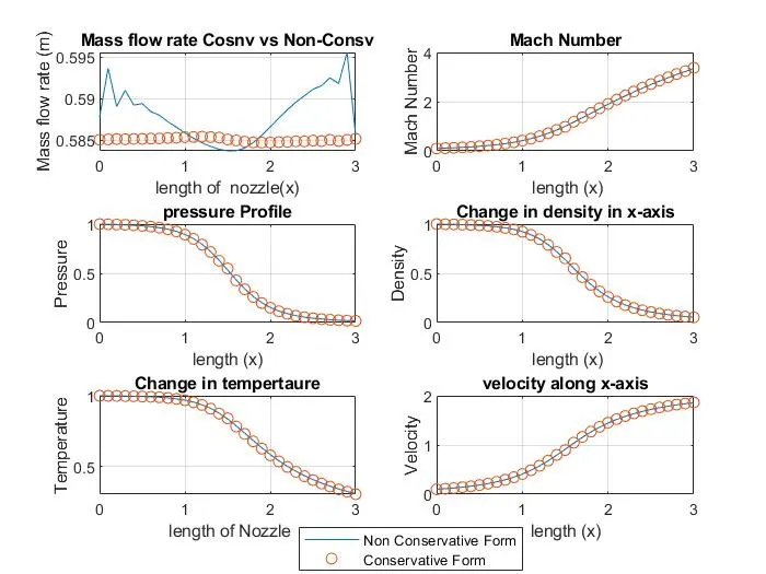
1. Change in Density,Mach number,Pressure,Velocity,Mass Flow Rate and Change in Temperature were compared for Conservative and Non conservative forms.As we see in the plots, that the profile for both conservative and Non conservative forms are same.
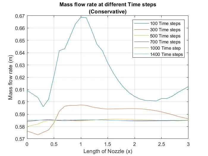
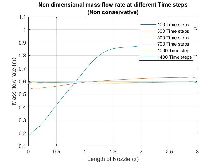
Except, Mass flow rate Comparision for both forms : The mass flow rate for conservative form along the length of nozzle shows the values are almost stable with less variations. The mass flow rate in non conservative form shows, becomes less at throat and varies .
2. Mass Flow Rate at different time steps for Conservative and Non- Conervative approach:
At inital time marching and the time derivatives are larger the values of mass flow rate is high throughout the nozzle.But after the 300 time steps , the values are comparitively approaching nearer to the expected analytical mark. After 700 time steps the mass flow is nearer to constant value. Comparing the mass flow rate of conservative with non-conservative form, the variations of mass flow are very less in conservative when inlet and oulet values are considered.
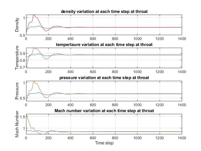
3.Mach number,Density,Pressure ,temperature for each time steps till 1400 time steps are plotted. Intially, the values of all the parameters(time derivatives) are very high and there are oscillations. These occur due to various effects caused by expansion and compression which occur in CD nozzle. Thereafter, the time steps values approach stability. The spikes are observed before 300 th time step. Minimum number of cycles should be run for simulation to converge is 600.
4.Grid Dependency Test
| Grid | rho1/rho0 | T1/T0 | P1/P0 |
| n=31 (Conservative) | 0.652 | 0.841 | 0.558 |
| n= 31(Non-Cons) | 0.639 | 0.836 | 0.554 |
| n= 101(Conservative) | 0.638 | 0.835 | 0.558 |
| n= 101(Non-Cons) | 0.638 | 0.836 | 0.552 |
Here rho1 ,P1 &T1 represents the values at throat. And rho0,P0&T0 represents the initial values at nozzle. The solutions are true for all locations within the nozzle. Even increasing the grid points did altered the solution marginally. Essentially solution is grid independent.
Conclusions:
- Solution converges after nearly around 700 time steps.
- Parameters like rho,P,T,V,Mach number are same for both the forms along the length of the nozzle.