Challenge

Week 5 - Mid term project - Solving the steady and unsteady 2D heat conduction problem

SSiddharth Banerjee26 Oct 2020

AIM:

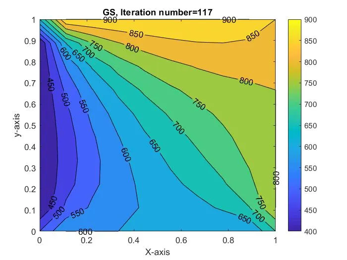
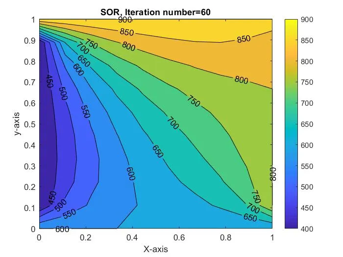
To solve 2D Heat conduction Partial Differential equation for steady and transient state using iterative techniques (a) Jacobi (b) Gauss Seidel (c)Successive over Relaxation (SOR) methods through MATLAB code.

Problem Definition

Heat conduction equation is defined by the general PDE:

α (∂²T/∂x² + ∂²T/∂y²+∂²T/∂z² )+ DT/Dt =0 , where alpha is known to be 'thermal diffusivity' (m^2/s)

Given that, the number of grid points in x direction is equal to y direction and the domain is assumed to be an unit squre.

Boundary conditions provided

1. Left (TL) = 400K 2. Right (TR) = 800K 3. Top(TT) = 600K 4. Bottom (TB) = 900K

1. Steady state analysis

The generalised 2D temperature Equation is for steady state analysis :

∂²T/∂x² + ∂²T/∂y²=0

**Point to note: The steady-state solution is a time-independent function. It is obtained by setting the partial derivative(s) with respect to t in the heat equation (or, later on, the wave equation) to constant zero, and then solving the equation for a function that depends only on the spatial variable x.

We discretize the eqn by central differencing,

The Eqn with respect to X becomes,

∂²T/∂x² = T(i−1,j) – 2 T (i,j) + T (i+1,j) / Δx²

The Eqn with respect to Y becomes,

∂²T/∂y²= T (i,j-1) − 2T (i,j)+T (i,j+1) / Δy²

Since we assumed, nx=ny then we can take , Δx²=Δy²

then the Eqn becomes as

T ⁿ⁺¹_(i,j) = 0.25* (T (i−1,j) + T (i+1,j) + T (i,j−1) + T (i,j+1)

%Solution for 2D Steady State Heat Conduction Eqn 
clear all 
close all
clc
% Steady-state Analysis: d^2T/dx^2+d^2/dy^2=0

% Inputs provided
L=1; % The domain is a unit square 
nx=10;
ny=nx; % grid points along x and y direction
dx=L/(nx-1); % change of x wrt x co-ordinate
dy= L/(ny-1); % change of y wrt y co-ordinate
x=linspace(0,1,nx);
y=linspace(0,1,ny);

% assigning boundary conditions 
% temperatures for steady and transient case
T_L=400;
T_T=600;
T_R=800;
T_B=900;
T=300*ones(nx,ny); % temperature array

% updating value of temperatures
T(:,1)=T_L;
T(:,nx)=T_R;
T(1,:)=T_T;
T(ny,:)=T_B;
Told=T;
% calculating average temperature at the matrix corners
T(1,1) = (T_T + T_L)/2;
T(nx,ny) = (T_R + T_B)/2;
T(1,ny) = (T_T + T_R)/2;
T(nx,1) = (T_L + T_B)/2;

iterative_solver=1;
error= 9e9;
tol=1e-4; %tolerance value

% jacobi method
  jacobi_iter=1;
  while(error>tol)
  for i=2:nx-1
   for j=2:ny-1
      T(i,j) = 0.25*((Told(i-1,j)+Told(i+1,j))) + 0.25*((Told(i,j-1)+Told(i,j+1)));
   end
  end
  error=max(max(abs(Told-T)));
  Told=T;
  jacobi_iter=jacobi_iter+1;
end

figure(1)
contourf(x,y,T,'ShowText','on');
colorbar;
title_text=sprintf('JACOBI, Iteration number=%d', jacobi_iter);
title(title_text);
xlabel('X-axis');
ylabel('y-axis');
pause(0.003);

% Gauss seidel method

% Inputs
L=1; % The domain is a unit square 
nx=10;
ny=nx; % grid points along x and y direction
dx=L/(nx-1); % change of x wrt x co-ordinate
dy= L/(ny-1); % change of y wrt y co-ordinate
x=linspace(0,1,nx);
y=linspace(0,1,ny);

% assigning boundary conditions 
% temperatures for steady and transient case
T_L=400;
T_T=600;
T_R=800;
T_B=900;
T=ones(nx,ny); % temperature array

% updating value of temperatures
T(:,1)=T_L;
T(:,nx)=T_R;
T(1,:)=T_T;
T(ny,:)=T_B;
Told=T;
% calculating average temperature at the matrix corners
T(1,1) = (T_T + T_L)/2;
T(nx,ny) = (T_R + T_B)/2;
T(1,ny) = (T_T + T_R)/2;
T(nx,1) = (T_L + T_B)/2;

error= 9e9;
tol=1e-4; %tolerance value

 gs_iter=1;
  while(error>tol)
  for i=2:nx-1
   for j=2:ny-1
      T(i,j) = 0.25*((T(i-1,j)+Told(i+1,j))) + 0.25*((T(i,j-1)+Told(i,j+1)));
   
    end
  end
  error=max(max(abs(Told-T)));
  Told=T;
  gs_iter=gs_iter+1;
  
 end

figure(2)
contourf(x,y,T,'ShowText','on');
colorbar;
title_text=sprintf('GS, Iteration number=%d', gs_iter);
title(title_text);
xlabel('X-axis');
ylabel('y-axis');
pause(0.003);

% Successive over relaxation method

% Inputs
L=1;  
nx=10;
ny=nx; % grid points along x and y direction
dx=L/(nx-1); % change of x wrt x co-ordinate
dy= L/(ny-1); % change of y wrt y co-ordinate
x=linspace(0,1,nx);
y=linspace(0,1,ny);

% assigning baundary conditions 
% temperatures for steady and transient case
T_L=400;
T_T=600;
T_R=800;
T_B=900;
T=300*ones(nx,ny); % temperature array
% calculating average temperature at the matrix corners
T(1,1) = (T_T + T_L)/2;
T(nx,ny) = (T_R + T_B)/2;
T(1,ny) = (T_T + T_R)/2;
T(nx,1) = (T_L + T_B)/2;

% updating value of temperatures
T(:,1)=T_L;
T(:,nx)=T_R;
T(1,:)=T_T;
T(ny,:)=T_B;
Told=T;

iterative_solver=1;
error= 9e9;
tol=1e-4; %tolerance value

  sor_iter=1;
  omega=1.3; % relaxation factor
  while(error>tol)
  for i=2:nx-1
   for j=2:ny-1
      T(i,j) =(1-omega)*Told(i,j)+omega*(0.25*((T(i-1,j)+Told(i+1,j))) + 0.25*((T(i,j-1)+Told(i,j+1))));
   
   end
 end
  error=max(max(abs(Told-T)));
  Told=T;
  sor_iter=sor_iter+1;
end

figure(3)
contourf(x,y,T,'ShowText','on');
colorbar;
title_text=sprintf('SOR, Iteration number=%d', sor_iter);
title(title_text);
xlabel('X-axis');
ylabel('y-axis');
pause(0.003);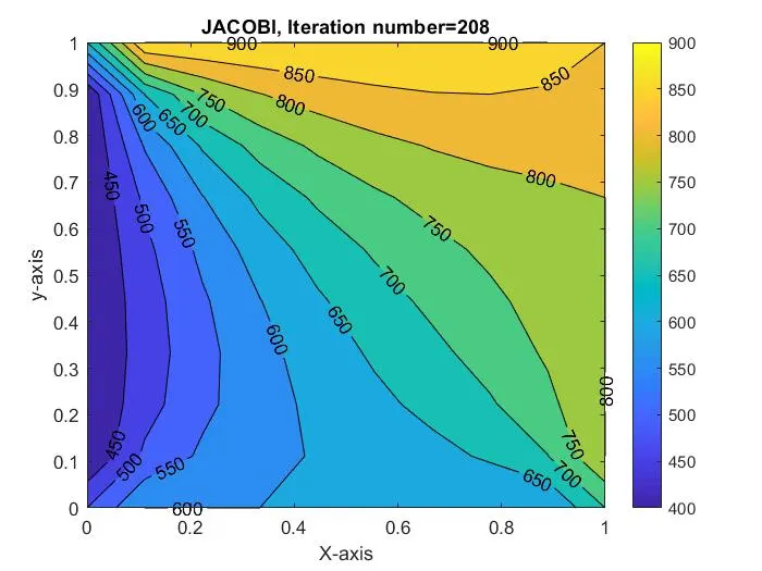

2.Transient State Analysis:

The generalised 2D temperature Equation is,

α (∂²T/∂x² + ∂²T/∂y²) + DT/Dt =0

Discretize the spatial part of eqn by (1) Central Differencing Scheme & (2)Time gradient Eqn with Forward Differencing Scheme

The Eqn with respect to X becomes,

∂2T/∂x2=T(i−1,j)−2T(i,j)+T(i+1,j) / Δx²

The Eqn with respect to Y becomes,

∂2T/∂y2=T(i,j-1)−2T(i,j)+T(i,j+1) / Δy²

The Eqn with respect to time gradient becomes

∂T/∂t =Tn+1(i,j)−Tn(i,j) / Δt

We can define 2 constants k1 and k2 as;

K1=αΔt/Δx²

K2=αΔt/Δy²

Since we assumed nx=ny then we can take Δx²=Δy²

then the Eqn becomes:

T ⁿ⁺¹_(i,j) =Tn(i,j)+k1[T(i−1,j)+T(i+1,j)] + k2[T(i,j−1)+T(i,j+1)] / (1+2K1+2K2)

close all
clear all
clc

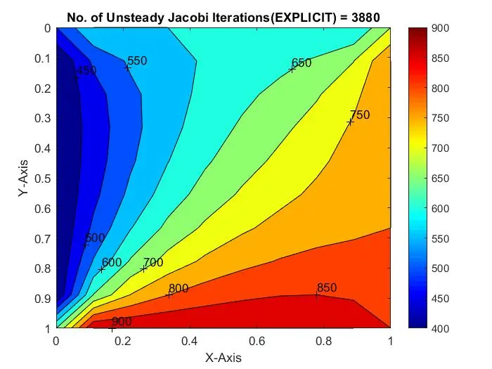
%Solving the Unsteady state 2D heat conduction by Jacobi Method(IMPLICIT SCHEME)

%Input Parameters
%Number of grid points
nx = 10;
ny = nx;
nt = 1400;

x = linspace(0,1,nx);
y = linspace(0,1,ny);

dx = x(2) - x(1);
dy = dx;

%Absolute error criteria > tolerance
error = 9e9;
tolerance = 1e-4;
dt = 1e-3;

%Defining Boundary conditions
T_L = 400;
T_T = 600;
T_R = 800;
T_B = 900;

T = 300*ones(nx,ny);

T(2:ny - 1, 1)  = T_L;
T(2:ny - 1, nx) = T_R;
T(1, 2:nx - 1)  = T_T;
T(ny, 2:nx - 1) = T_B;

%Calculating Average temperature at corners
T(1,1) = (T_T + T_L)/2;
T(nx,ny) = (T_R + T_B)/2;
T(1,ny) = (T_T + T_R)/2;
T(nx,1) = (T_L + T_B)/2;

%Assigning orginal values to T
T_old = T;
T_intial = T;

%Calculation of 2D steady heat conduction EQUATION by Successive over-relaxation method
k1 = 1.1*(dt/(dx^2));
k2 = 1.1*(dt/(dy^2));

Jacobi_iteration = 1;
for k = 1:nt
    error = 9e9; 
    
    while(error > tolerance)
        
        for i = 2:nx - 1
            
            for j = 2:ny - 1
                    
                Term_1 = 1/(1 + (2*k1) + (2*k2));
                Term_2 = k1*Term_1;
                Term_3 = k2*Term_1;
                H = (T_old(i-1,j)) + (T_old(i+1,j));
                V = (T_old(i,j+1)) + (T_old(i,j-1));
                    
                T(i,j) = (T_intial(i,j)*Term_1) + (H*Term_2) + (V*Term_3);
   
            end
            
        end
        
        error = max(max(abs(T_old - T)));
        T_old = T;
        Jacobi_iteration = Jacobi_iteration + 1;  
        
    end
    
    T_intial = T;
    
    %Plotting
    figure(1)
    contourf(x,y,T)
    clabel(contourf(x,y,T))
    colorbar
    colormap(jet)
    set(gca, 'ydir', 'reverse')
    xlabel('X-Axis')
    ylabel('Y-Axis')
    title(sprintf('No. of Unsteady Jacobi Iterations(EXPLICIT) = %d', Jacobi_iteration));
    pause(0.03)
end


%Solving the Unsteady state 2D heat conduction by Gauss Seidel Method(IMPLICIT SCHEME)

%Input Parameters
%Number of grid points
nx = 10;
ny = nx;
nt = 1400;

x = linspace(0,1,nx);
y = linspace(0,1,ny);

dx = x(2) - x(1);
dy = dx;

%Absolute error criteria > tolerance
error = 9e9;
tolerance = 1e-4;
dt = 1e-3;

%Defining Boundary conditions
T_L = 400;
T_T = 600;
T_R = 800;
T_B = 900;

T = 300*ones(nx,ny);

T(2:ny - 1, 1)  = T_L;
T(2:ny - 1, nx) = T_R;
T(1, 2:nx - 1)  = T_T;
T(ny, 2:nx - 1) = T_B;

%Calculating Average temperature at corners
T(1,1) = (T_T + T_L)/2;
T(nx,ny) = (T_R + T_B)/2;
T(1,ny) = (T_T + T_R)/2;
T(nx,1) = (T_L + T_B)/2;

%Assigning orginal values to T
T_old = T;
T_intial = T;

%Calculation of 2D steady heat conduction EQUATION by Successive over-relaxation method
k1 = 1.1*(dt/(dx^2));
k2 = 1.1*(dt/(dy^2));

Gauss_Seidel_iteration = 1;
for k = 1:nt
    error = 9e9; 
    
    while(error > tolerance)
        
        for i = 2:nx - 1
            
            for j = 2:ny - 1
                    
                Term_1 = 1/(1 + (2*k1) + (2*k2));
                Term_2 = k1*Term_1;
                Term_3 = k2*Term_1;
                H = (T(i-1,j)) + (T_old(i+1,j));
                V = (T(i,j+1)) + (T_old(i,j-1));
                    
                T(i,j) = (T_intial(i,j)*Term_1) + (H*Term_2) + (V*Term_3);
   
            end
            
        end
        
        error = max(max(abs(T_old - T)));
        T_old = T;
        Gauss_Seidel_iteration = Gauss_Seidel_iteration + 1;  
        
    end
    
    T_intial = T;
    
    %Plotting
    figure(1)
    contourf(x,y,T)
    clabel(contourf(x,y,T))
    colorbar
    colormap(jet)
    set(gca, 'ydir', 'reverse')
    xlabel('X-Axis')
    ylabel('Y-Axis')
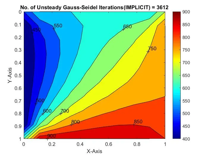
    title(sprintf('No. of Unsteady Gauss-Seidel Iterations(IMPLICIT) = %d', Gauss_Seidel_iteration));
    pause(0.03)
end

close all
clear all
clc

%Solving the Unsteady state 2D heat conduction by Successive over-relaxation Method(IMPLICIT SCHEME)

%Input Parameters
%Number of grid points
nx = 10;
ny = nx;
nt = 1400;

x = linspace(0,1,nx);
y = linspace(0,1,ny);

dx = x(2) - x(1);
dy = dx;

%Absolute error criteria > tolerance
error = 9e9;
tolerance = 1e-4;
dt = 1e-3;
omega = 1.1;

%Defining Boundary conditions
T_L = 400;
T_T = 600;
T_R = 800;
T_B = 900;

T = 300*ones(nx,ny);

T(2:ny - 1, 1)  = T_L;
T(2:ny - 1, nx) = T_R;
T(1, 2:nx - 1)  = T_T;
T(ny, 2:nx - 1) = T_B;

%Calculating Average temperature at corners
T(1,1) = (T_T + T_L)/2;
T(nx,ny) = (T_R + T_B)/2;
T(1,ny) = (T_T + T_R)/2;
T(nx,1) = (T_L + T_B)/2;

%Assigning orginal values to T
T_old = T;
T_intial = T;
T_end = T;

%Calculation of 2D steady heat conduction EQUATION by Successive over-relaxation method
k1 = 1.1*(dt/(dx^2));
k2 = 1.1*(dt/(dy^2));

Successive_over_relaxation_iteration = 1;
for k = 1:nt
    error = 9e9; 
    
    while(error > tolerance)
        
        for i = 2:nx - 1
            
            for j = 2:ny - 1
                    
                Term_1 = 1/(1 + (2*k1) + (2*k2));
                Term_2 = k1*Term_1;
                Term_3 = k2*Term_1;
                H = (T(i-1,j)) + (T_old(i+1,j));
                V = (T(i,j+1)) + (T_old(i,j-1));
                    
                T(i,j) = (T_intial(i,j)*Term_1) + (H*Term_2) + (V*Term_3);
                T_end(i,j) = ((1-omega)*T_old(i,j)) + (T(i,j)*omega);
                
            end
            
        end
        
        error = max(max(abs(T_old - T)));
        T_old = T_end;
        Successive_over_relaxation_iteration = Successive_over_relaxation_iteration + 1;  
        
    end
    
    T_intial = T_end;
    
    %Plotting
    figure(1)
    contourf(x,y,T)
    clabel(contourf(x,y,T))
    colorbar
    colormap(jet)
    set(gca, 'ydir', 'reverse')
    xlabel('X-Axis')
    ylabel('Y-Axis')
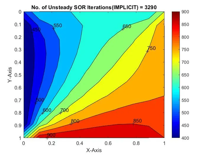
    title(sprintf('No. of Unsteady SOR Iterations(IMPLICIT) = %d', Successive_over_relaxation_iteration));
    pause(0.03)
end

close all
clear all
clc

%Solving the Unsteady state 2D heat conduction (EXPLICIT SCHEME)

%Input Parameters
%Number of grid points
nx = 10;
ny = nx;
nt = 1400;

x = linspace(0,1,nx);
y = linspace(0,1,ny);

dx = x(2) - x(1);
dy = dx;

%Absolute error criteria > tolerance
error = 9e9;
tolerance = 1e-4;
dt = 1e-3;
omega = 1.1;

%Defining Boundary conditions
T_L = 400;
T_T = 600;
T_R = 800;
T_B = 900;

T = 300*ones(nx,ny);

T(2:ny - 1, 1)  = T_L;
T(2:ny - 1, nx) = T_R;
T(1, 2:nx - 1)  = T_T;
T(ny, 2:nx - 1) = T_B;

%Calculating Average temperature at corners
T(1,1) = (T_T + T_L)/2;
T(nx,ny) = (T_R + T_B)/2;
T(1,ny) = (T_T + T_R)/2;
T(nx,1) = (T_L + T_B)/2;

%Assigning orginal values to T
T_intial = T;
T_old = T;


%Calculation of 2D steady heat conduction EQUATION by Successive over-relaxation method
iterative_solver = 1;
k1 = 1.1*(dt/(dx^2));
k2 = 1.1*(dt/(dy^2));

if iterative_solver == 1
    Steady_Explicit = 1;
    for k = 1:nt
        error = 1; 
    
        while(error > tolerance)
        
            for i = 2:nx - 1
            
                for j = 2:ny - 1
                    Term_1 = T_old(i,j);
                    Term_2 = k1*(T_old(i+1,j) - 2*T_old(i,j) + (T_old(i-1,j)));
                    Term_3 = k2*(T_old(i,j+1) - 2*T_old(i,j) + T_old(i,j-1));
                    T(i,j) = Term_1 + Term_2 + Term_3;
                end
            
            end
        
            error = max(max(abs(T_old - T)));
            T_old = T;
            Steady_Explicit = Steady_Explicit + 1;  
        
        end
    end
end

%Plotting
figure(1)
contourf(x,y,T)
clabel(contourf(x,y,T))
colorbar
colormap(jet)
set(gca, 'ydir', 'reverse')
xlabel('X-Axis')
ylabel('Y-Axis')
title(sprintf('No. of Unsteady Iterations(EXPLICIT) = %d', Steady_Explicit));
pause(0.03);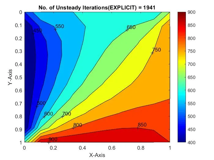

3. Result Review

Steady Flow Iterative Solver
Method	No. of iterations	Error value
Jacobi	208	1.5830e-04
Gauss-Seidel	117	1.2290e-04
SOR	60	9.5421e-05
Transient Flow Iterative Solver (Implicit)
Method	No. of iterations	Error value
Jacobi	3880	1.6124e-04
Gauss-Seidel	3612	1.2715e-04
SOR	3290	9.6875e-05

=> From the above table, we conclude that the Successive over-relaxation Iterative method proves to be providing results converging towards the solution with fewer numbers of iterative cycles with minimum error values.

=> SUCCESSIVE OVER RELAXATION Method proves to be the Cost & time effective method when compared to Jacobi & Gauss-Seidel iterative Methods.

=> Explicit Scheme requires excessively large number of iterations to converge on a solution, which is impractical considering the lower number of iterations required in Implicit Scheme. Explicit is said to favor time accurate solutions largely.

Week 5 - Mid term project - Solving the steady and unsteady 2D heat conduction problem

Ship work like this
in your own course.

Talk to a career counsellor

Ship work like thisin your own course.

Talk to a career counsellor

Ship work like this
in your own course.