Steady Vs Unsteady flow over a cylinder

Aim

• Part 1: Simulate the flow with the steady and unsteady case and calculate the Strouhal Number for Re= 100.
• Part 2: a) Calculate the coefficient of drag and lift over a cylinder by setting the Reynolds number to 10, 100, 1000, 10000 & 100000. (steady state solver) b) Discuss the effect of Reynolds number on the coefficient of drag.[Results should be validated with any standard literature & error must be within 5%.

Introduction:

1. Analysing the flow over a cylinder helps to study the effects of vortex shedding in steady state and in transient state simulations.
2. Vortex shedding is an unsteady flow that takes place in a special flow velocities (according to size and shape of the cylindrical body).
3. In this flow, vortices are created at the back of the body and detach periodically from either side of the body.
4. Vortex shedding is an effect of : Viscosity and Reynolds number. It mainly depends up on velocity of the fluid, type of fluid, and shape of the respective objective.
5. In this flow, vortices are created at the back of the body and detach periodically from either side of the body.
6. Generally vortex shedding occurs above a particular value of Reynolds number, where Reynolds number is represented by Re=(ρ*u*D)/μ). Here ρ = density, u = velocity, D = diameter, μ = absolute viscosity.
7. Vortex shedding is basically given by Strouhal Number(st) i.e. St = (f*D)/u, where f = frequency of shedding, D = diameter, u = velocity of fluid.

1. Simulate the flow with the steady and unsteady case and calculate the Strouhal Number for Re= 100.

a) Construction of the cylinder using Space Claim

2 m dia cylinder

Creation of Enclosure Volume

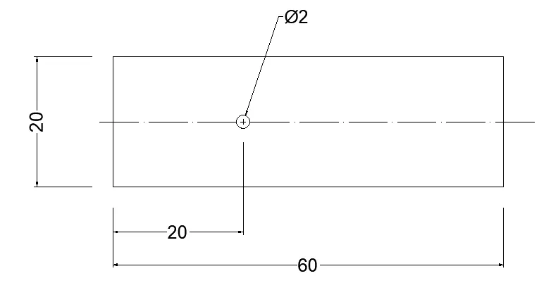
Dimensions of the setup (in m)

b) Meshing of the Enclosure

> Named Selection representing the setup

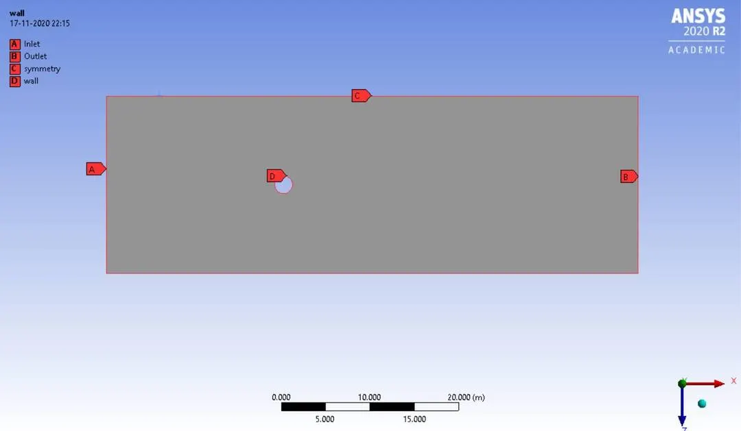
> The model was meshed using element size of 0.25 m (simulation done with this element size)

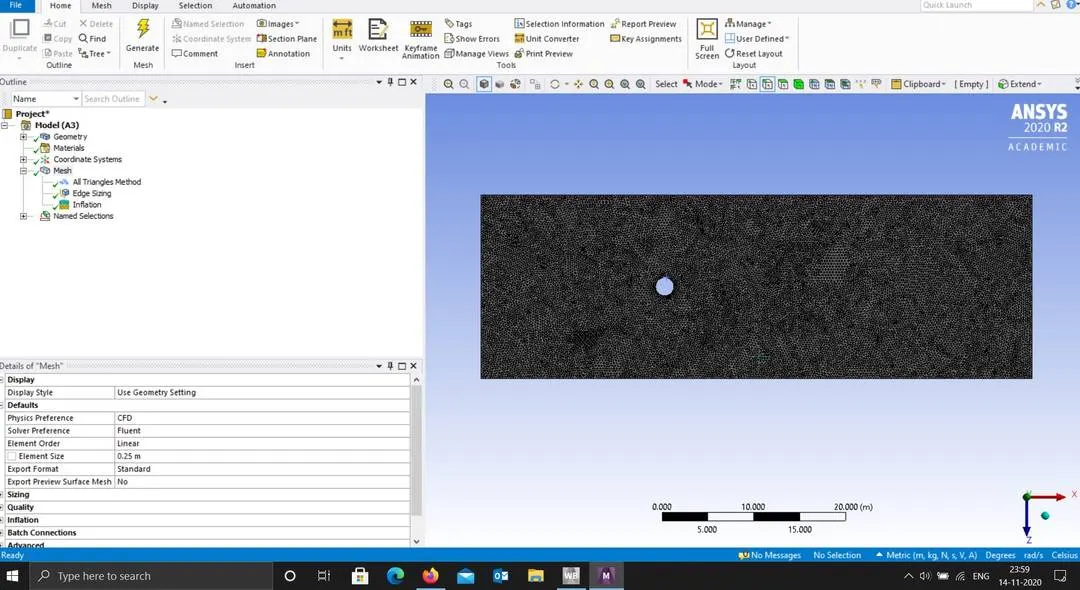
The additional refinements done to capture flow of air around cylinder wall wer as follows:

1. Local mesh refinement was further done by using triangular method for proper meshing(smoothening) of the hole

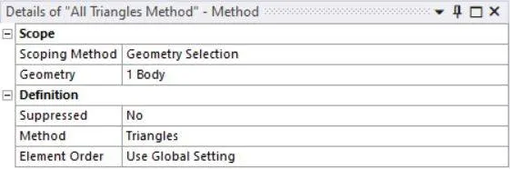
2. Edge sizing was to the cylinder wall edge.

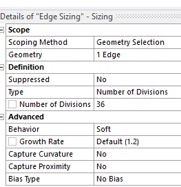
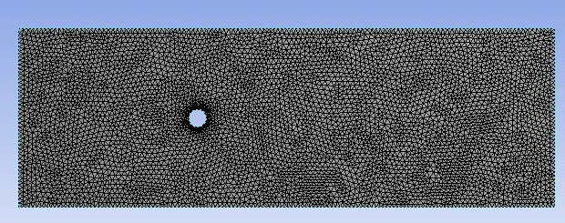
3.To capture the no-slip conditions properly inflation layer is set up.

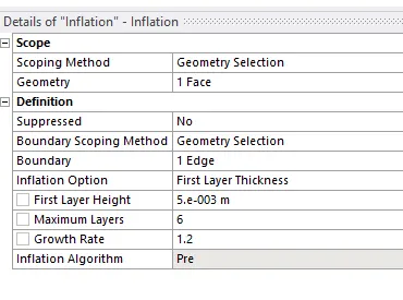
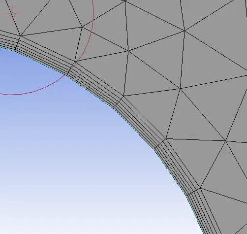
** The quality of mesh was checked using mesh metric and result are acceptable for this simulations.

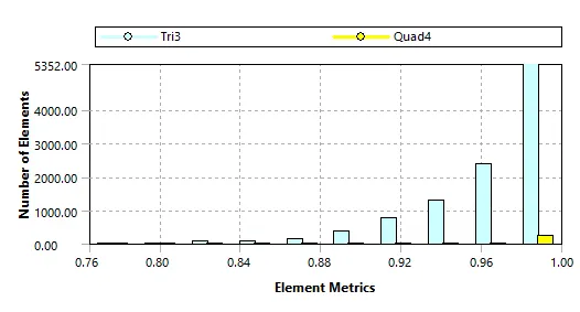
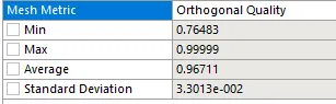
Fig: Orthogonal Quality

c) Reference Values and Setup

In fluent setup we will be running steady and transient case of this problem. As, the flow is laminar, so we will be using a viscous-laminar model for this simulations.

------------------------------------------------------------------------------

Materials : air

Properties: -density= 1kg/m^3 -viscosity=0.02 (kg/m-s)

For boundary conditions:

-Velocity inlet: 0.1,1,10,100,1000 m/s (for all the cases)

-Outlet pressure: 0 Pa

-Wall: No slip condition

> A monitor point is setup at locations (8,0) to monitor velocity and pressure behind the cylinder wall.

Part 1 : Simulate the flow with the steady and unsteady case and calculate the Strouhal Number for Re= 100.

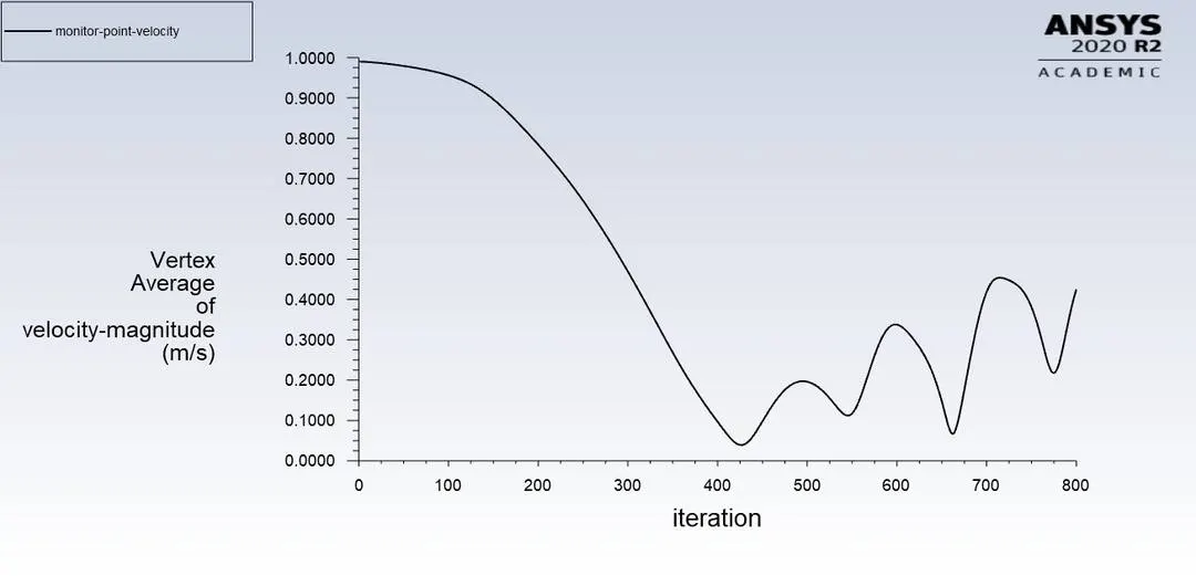
For steady state with RE=100 and inlet velocity =1 m/s the simulations was carried using 500 time step. For transient state with RE=100 and inlet velocity=1m/s the simulation was carried using at time steps size of 0.1 sec with 1200 no. of time steps which gives us simulation time of 120sec.The reference value were set before running the simulations to avoid any wrong result. The reference data is shown below.

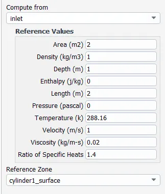
For the remaining simulation all the values will be kept same, except for the velocity which we need to change accordingly with RE no.

> In order to calculate the vortex shedding for the different reynolds number we have to calculate the velocity for that particular reynolds number :

Now we know that the reynolds number is given by :

Re = (Dia of cylinder * velocity) / Kinematic Viscousity

Therefore the velocity for Re = 100 is given by :

Velocity ~= 0.02 *100 / 2

= 1 m/s , similarly Free Steam Vel is computed for to achieve varied Reynolds No.

RESULT & PLOTS

STEADY STATE SOLVER TURBULENT SOLVER

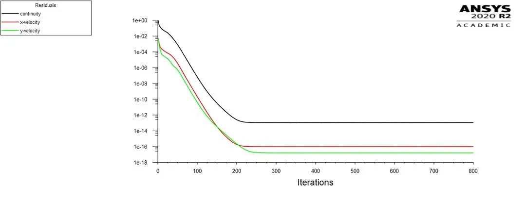
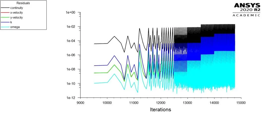
a)Residuals

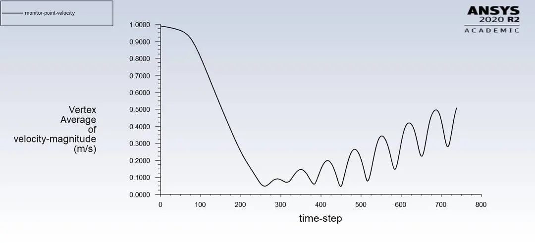
b)Monitor Point Velocity

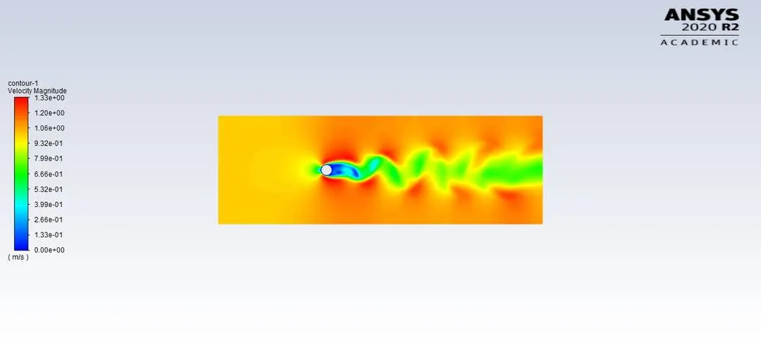
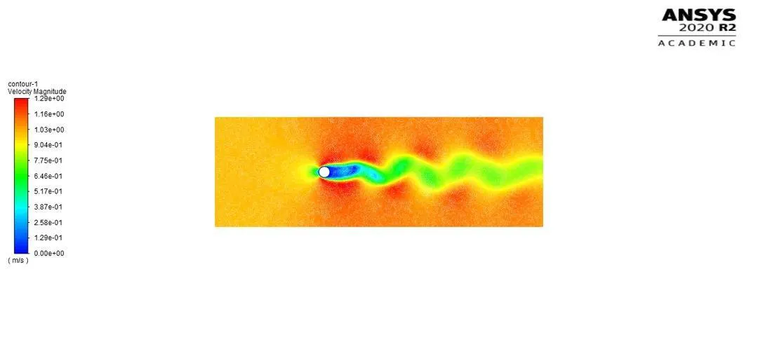
c) Velocity Contour

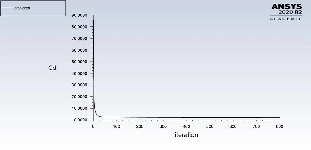
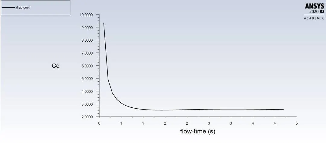
d) Drag Coeff

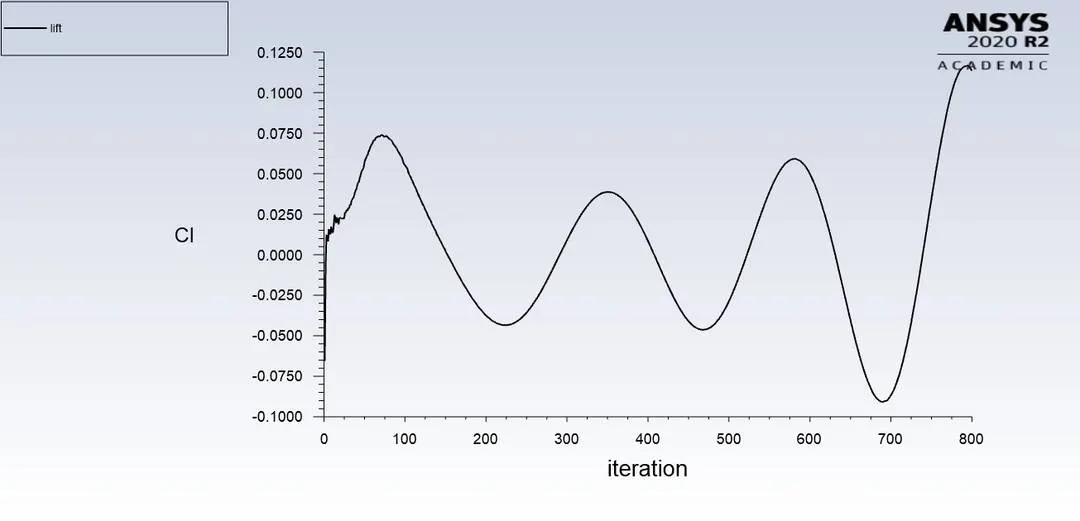
e) Lift

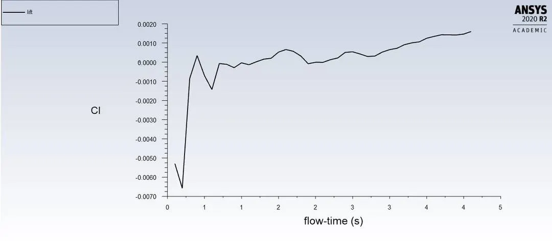
f) Pressure Contour

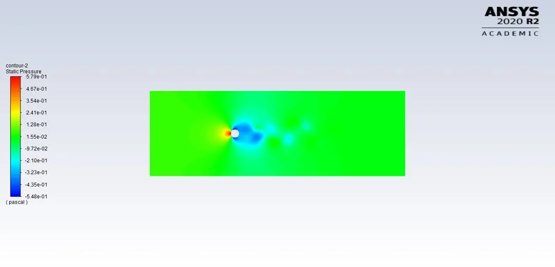
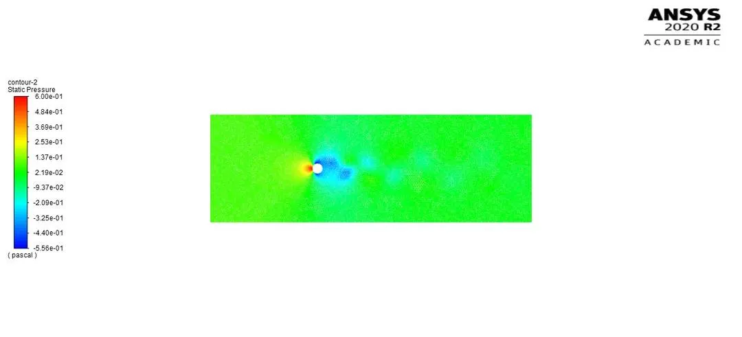
Now we will be defining strouhal number as below :

The Strouhal Number is a dimensionless value useful for analyzing oscillating unsteady fluid flow dynamics problems.

The Strouhal Number can be expressed as

St = ω l / v

where

St = Strouhal Number

ω = oscillation frequency

l = characteristic length

v = flow velocity

The Strouhal Number represents a measure of the ratio of the inertial forces due to the unsteadiness of the flow or local acceleration to the inertial forces due to changes in velocity from one point to an other in the flow field.

For Case 1 : Strouhal Number

Now we know that the frequency = no of cycles / time change

Therefore frequency = 2 / 662-550 ( time step values from Turbulent monitor point velocity plot)

= 2/ [(212*0.1) in seconds ; Time Step Size=0.1 ]

= .0943 hz

Therefore, St = 0.0943 *2 / 1

= 0.1886

• Strouhal Number is directly praportional on the frequency of Vortex Shedding.
• In steady state analysis we cannot find the frequency as there is no time parameter involved , where as in case of transient Analysis we can find the frequency.

Re=100 , Turbulent Solver GIF

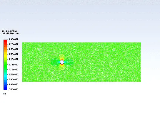
Vortex Shredding Explained as observed above

As a fluid particle flows toward the leading edge of a cylinder, the pressure on the particle rises from the free stream pressure to the stagnation pressure. The high fluid pressure near the leading edge impels flow about the cylinder as boundary layers develop about both sides. The high pressure is not sufficient to force the flow about the back of the cylinder at high Reynolds numbers. Near the widest section of the cylinder, the boundary layers separate from each side of the cylinder surface and form two shear layers that trail aft in the flow and bound the wake. Since the innermost portion of the shear layers, which is in contact with the cylinder, moves much more slowly than the outermost portion of the shear layers, which is in contact with the free flow, the shear layers roll into the near wake, where they fold on each other and coalesce into discrete swirling vortices. A regular pattern of vortices called a vortex street trails aft in the wake.

Part 2

a) Coefficient of Drag and Coefficient of Lift plot by setting the Reynolds number to 10,100,1000,10000 & 100000.

• Coefficient of Drag:
  The aerodynamic drag coefficient is a measure of the effectiveness of a streamline aerodynamic body shape in reducing the air resistance to the forward motion of a vehicle. A low drag coefficient implies that the streamline shape of the vehicle's body is such as to enable it to move easily through the surrounding viscous air with the minimum of resistance; conversely, a high drag coefficient is caused by poor streamlining of the body profile so that there is a high air resistance when the vehicle is in motion.

C_d is given by,

C_d=2F_d / (ρ⋅u²⋅A)

where, F_d - implies to the Net backward force.

• Coefficient of Lift:
  The lift coefficient (C_L) is a dimensionless coefficient that relates the lift generated by a lifting body to the fluid density around the body, the fluid velocity, and an associated reference area.

C_l is given by,

C_l=2F_l / (ρ⋅u²⋅A)

where, F_l - implies to the Net Upward force.

Case1:

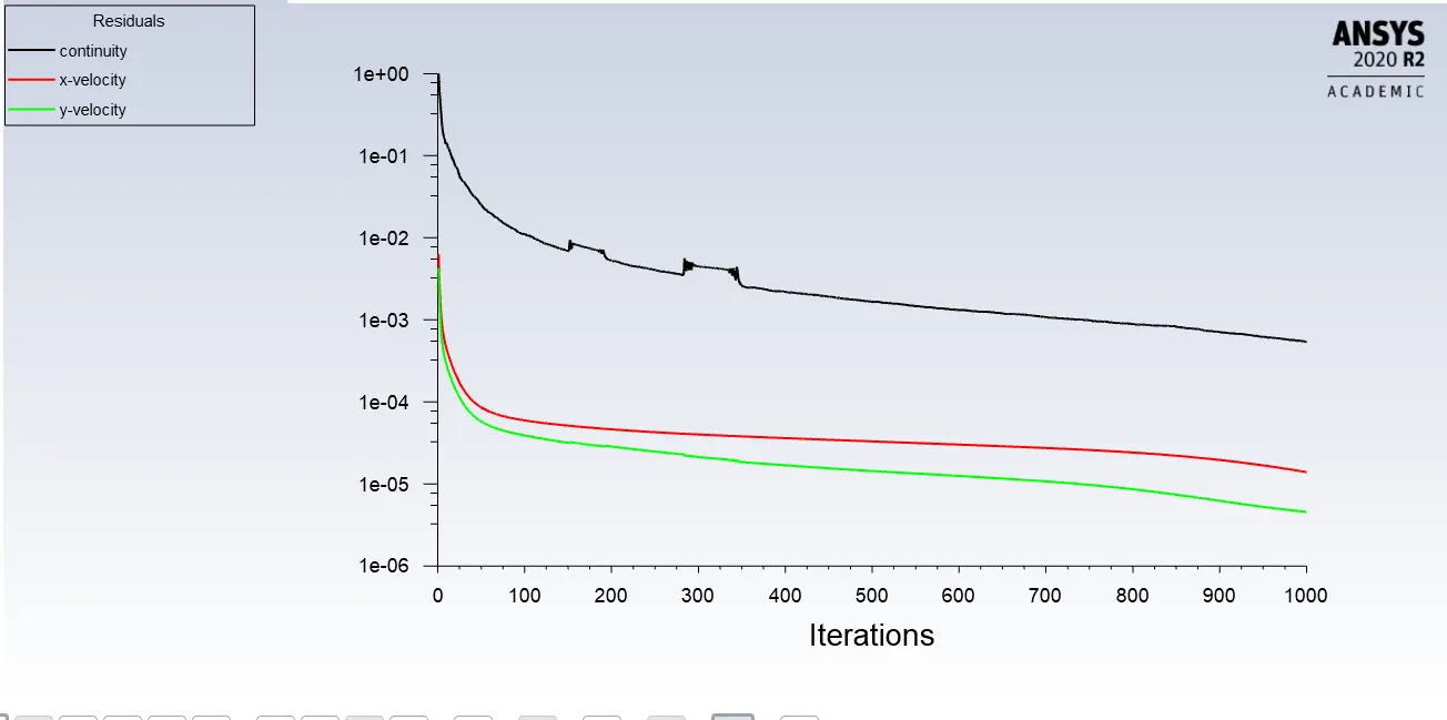
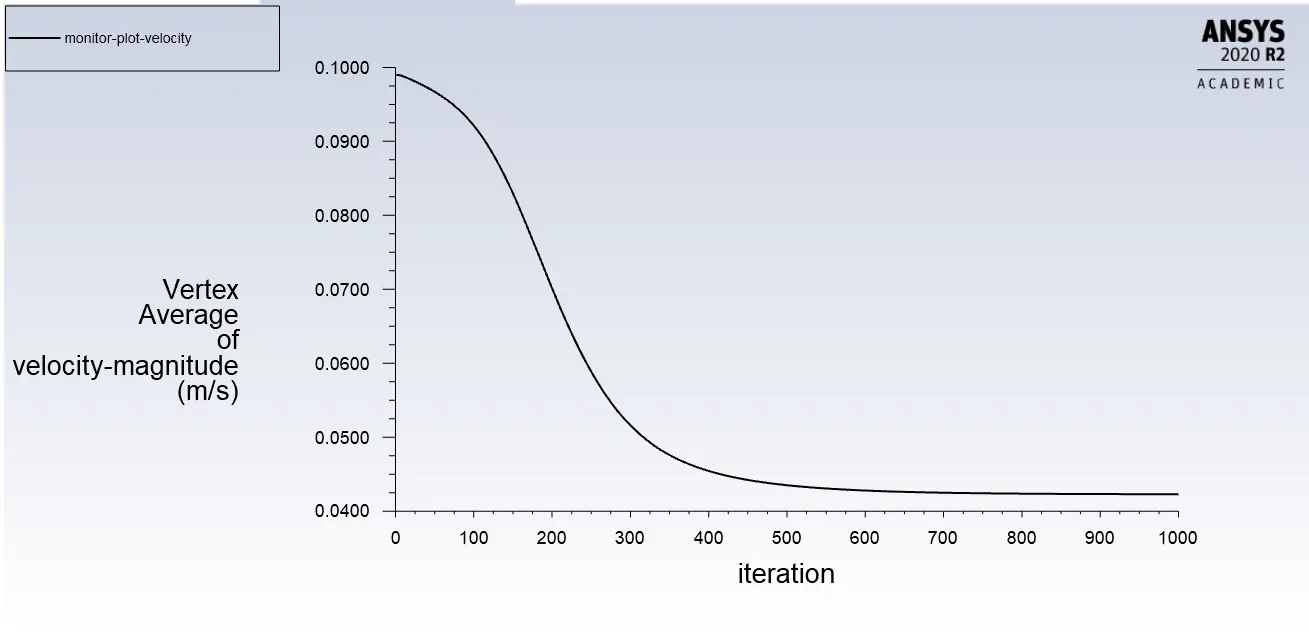
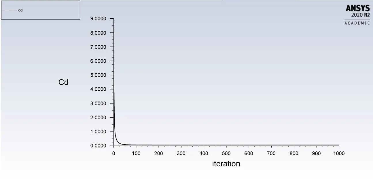
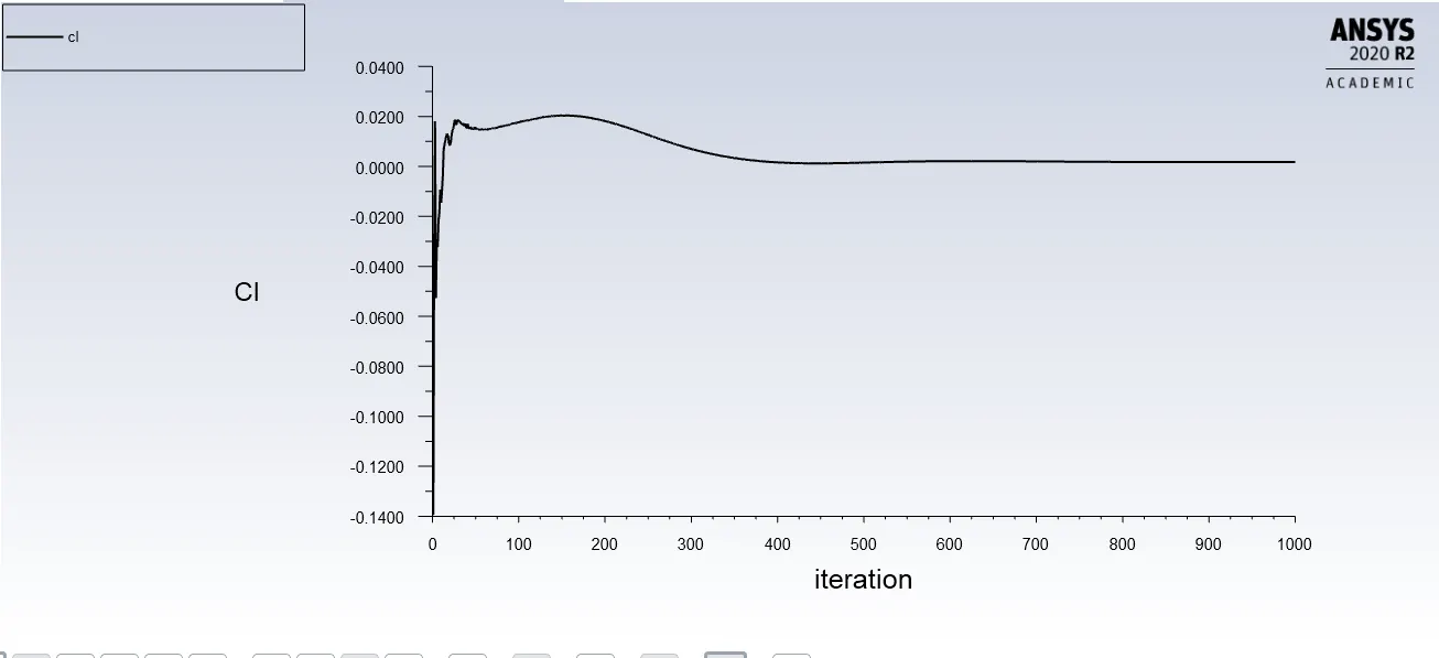
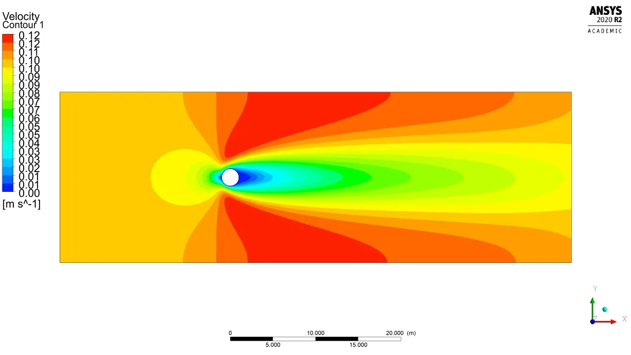
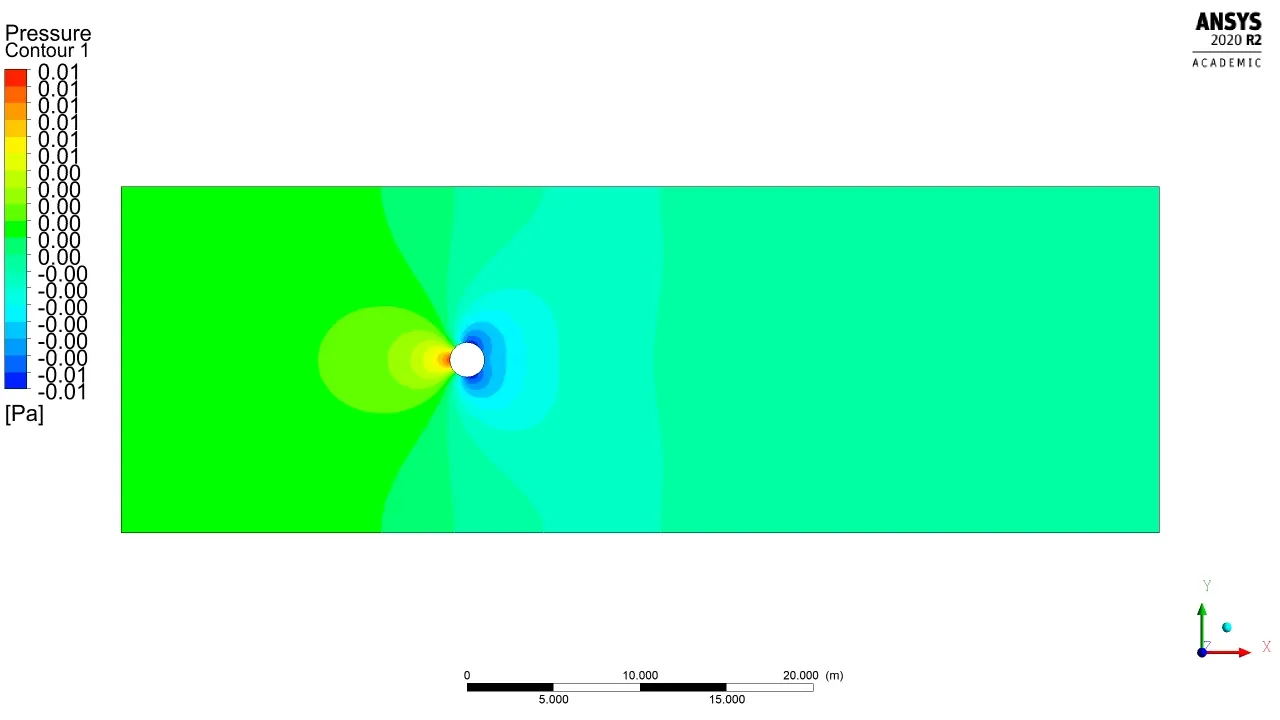
Reynolds Number = 10

viscosity = 0.02

Velocity = 0.1

Iterations = 1000

Residual plot:

Monitor point velocity:

Drag Coefficient:

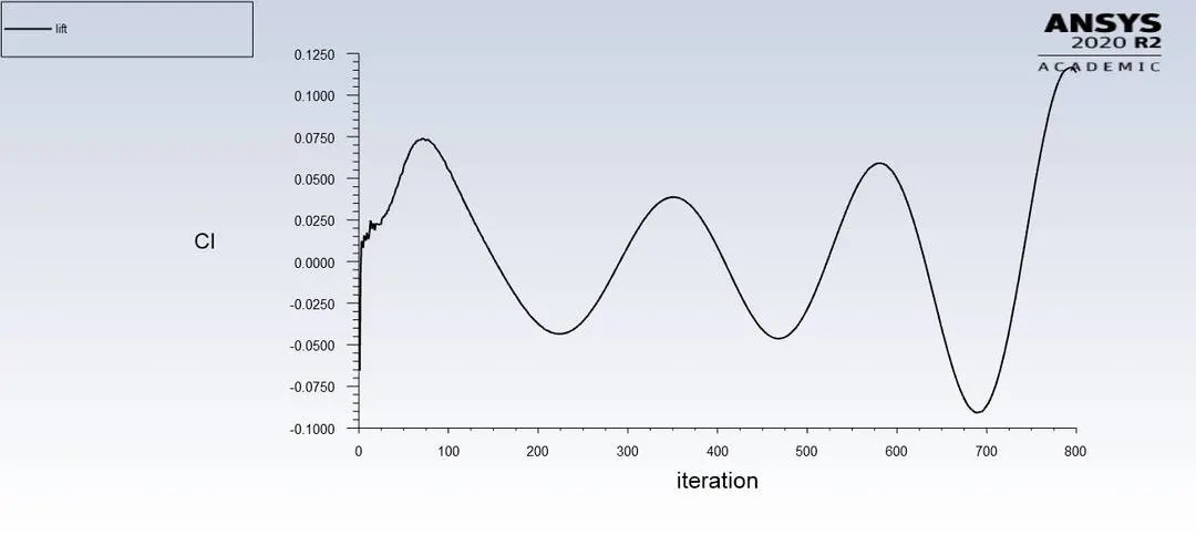
Lift coefficient:

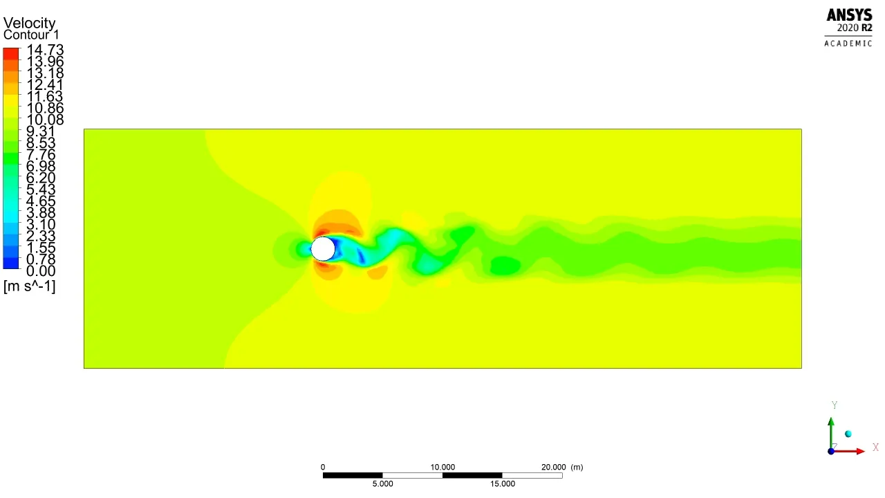
Velocity contour:

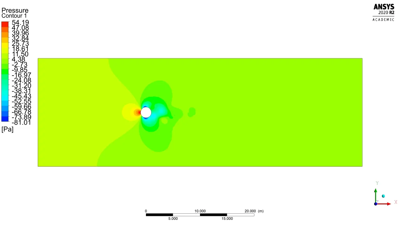
Pressure contour:

Case 2 :

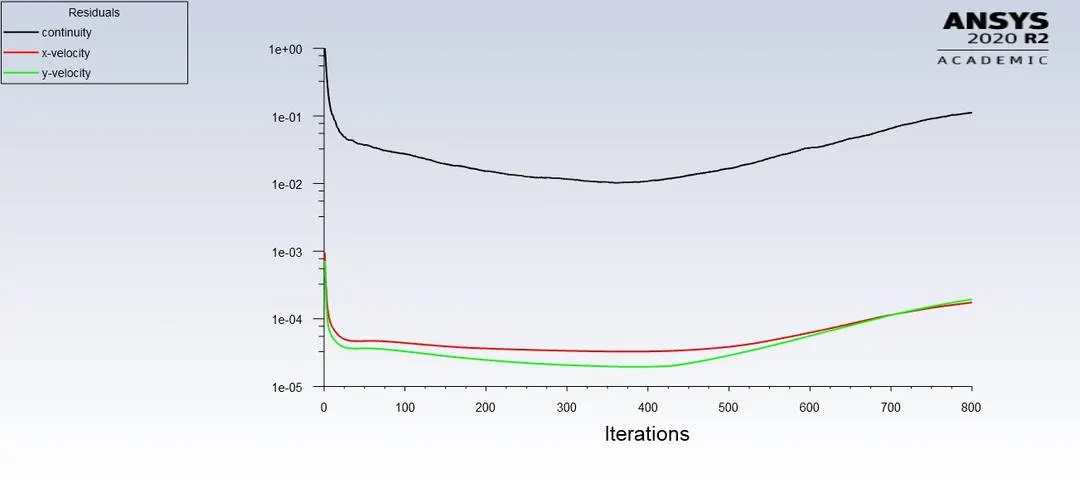
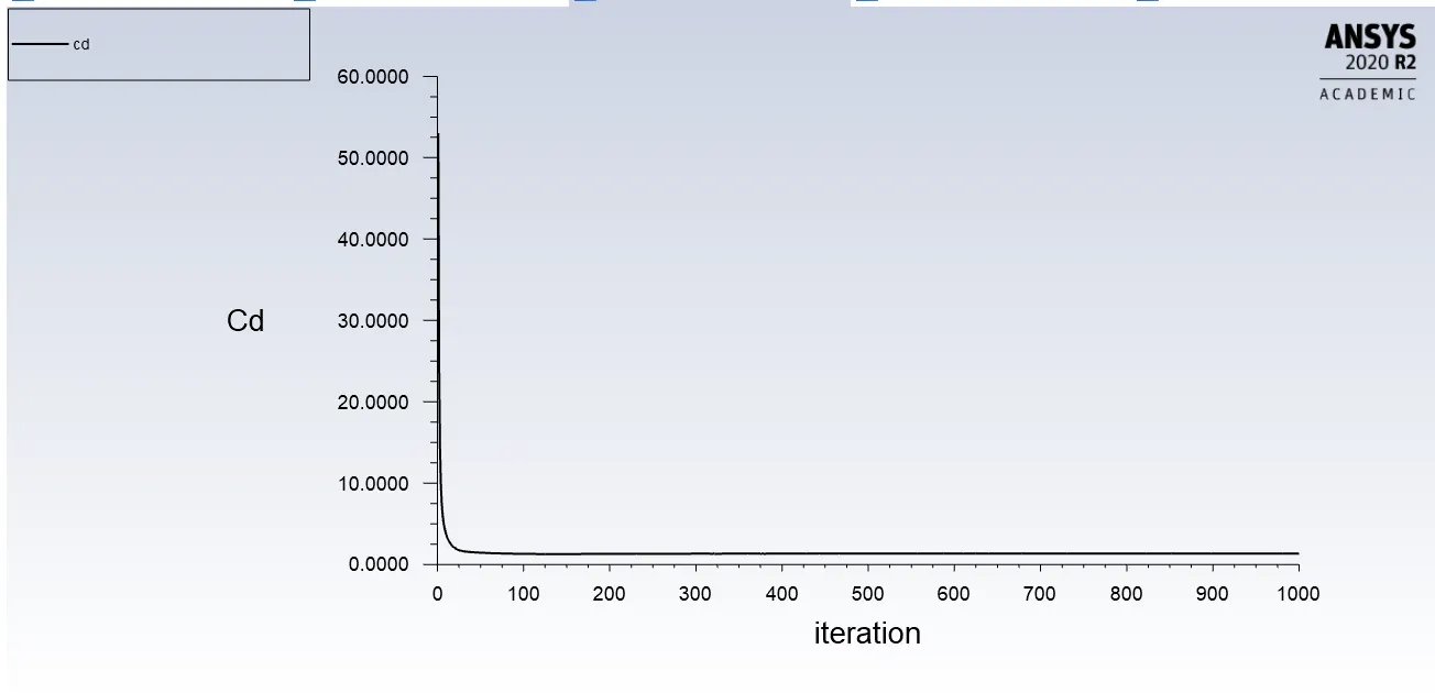
Reynolds number: 100

velocity: 1

viscosity: 0.02

Iterations: 1000

Residual plot:

Monitor point velocity:

Drag Coefficient:

Lift coefficient:

Velocity contour:

Pressure contour:

Case 3:

Reynolds number: 1000

Velocity: 10

viscosity : 0.02

Iterations: 1000

Residual plot:

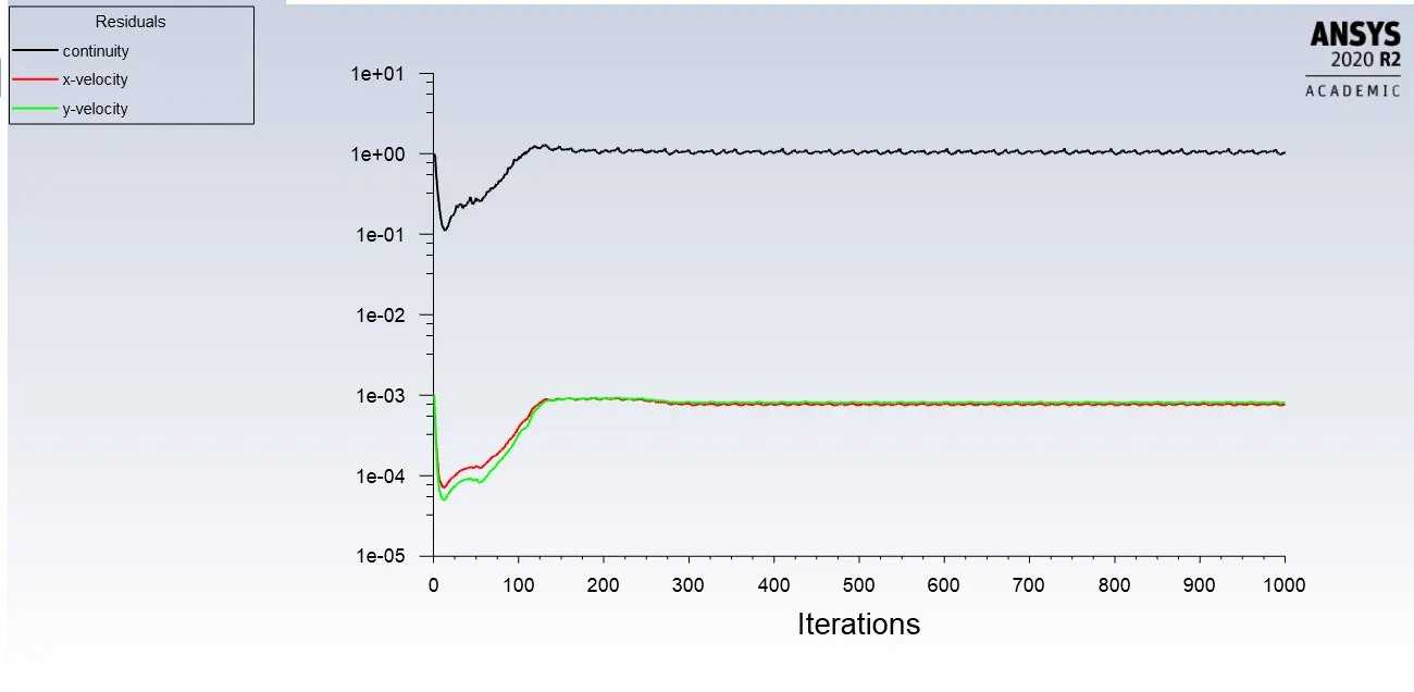
Monitor point velocity:

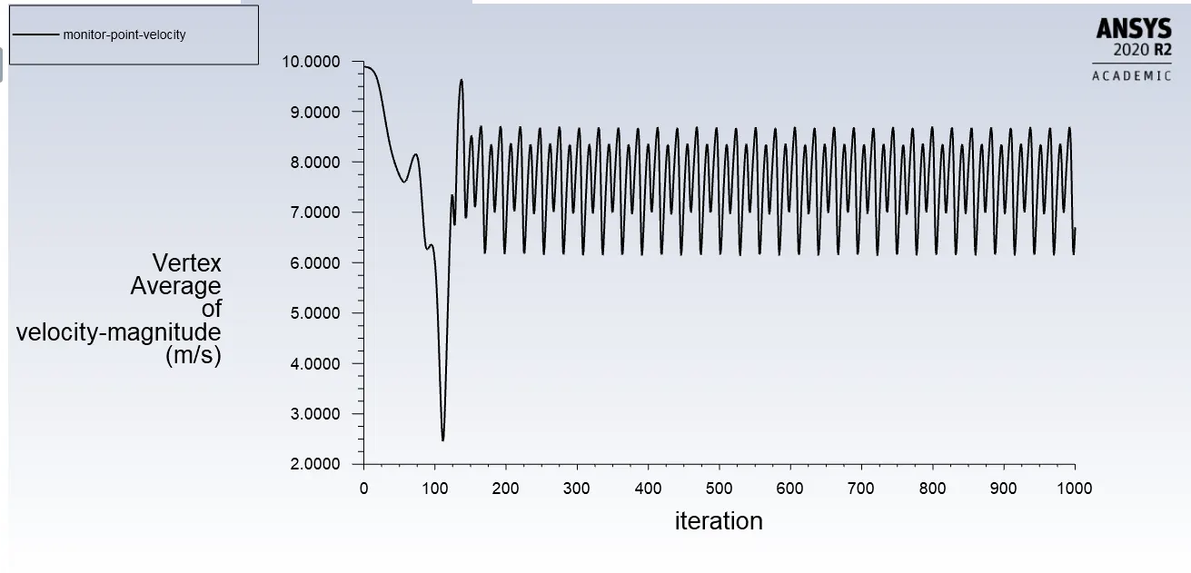
Drag Coefficient:

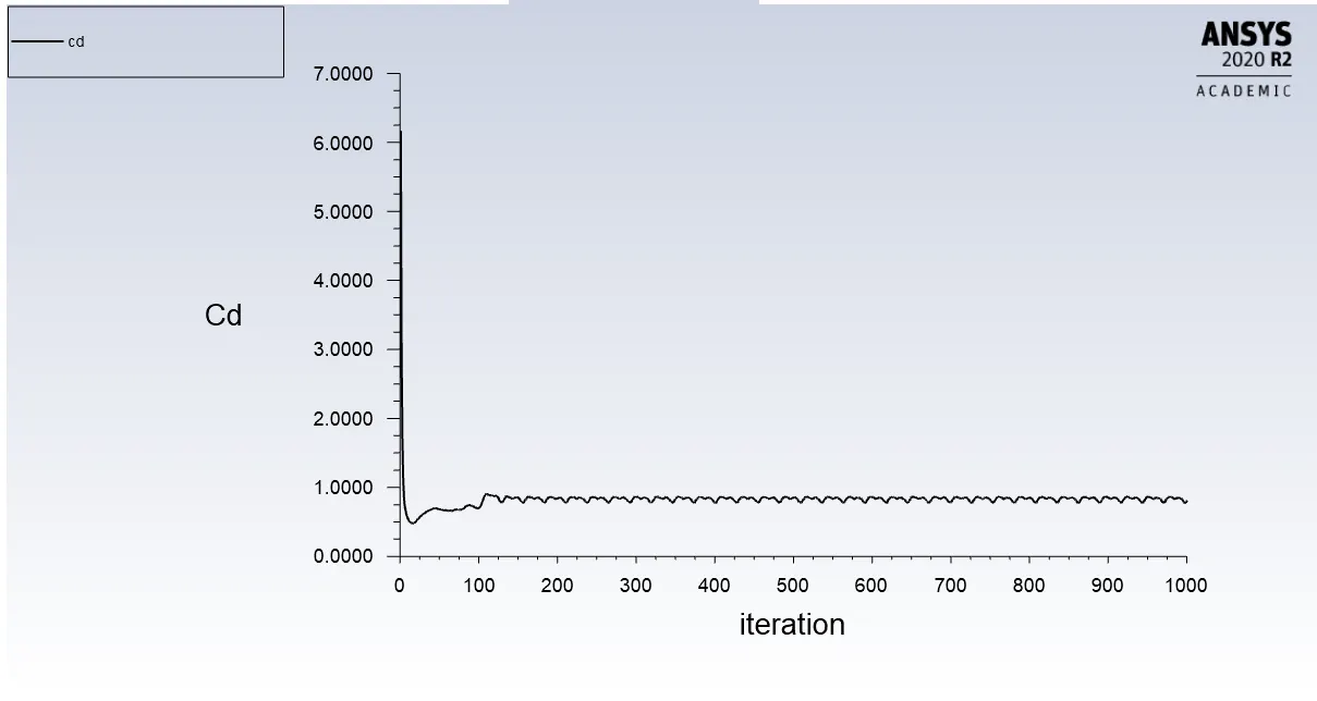
Lift coefficient:

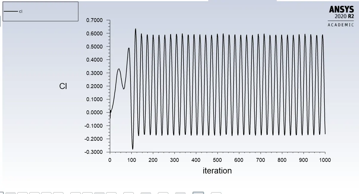
Velocity contour:

Pressure contour:

Case 4:

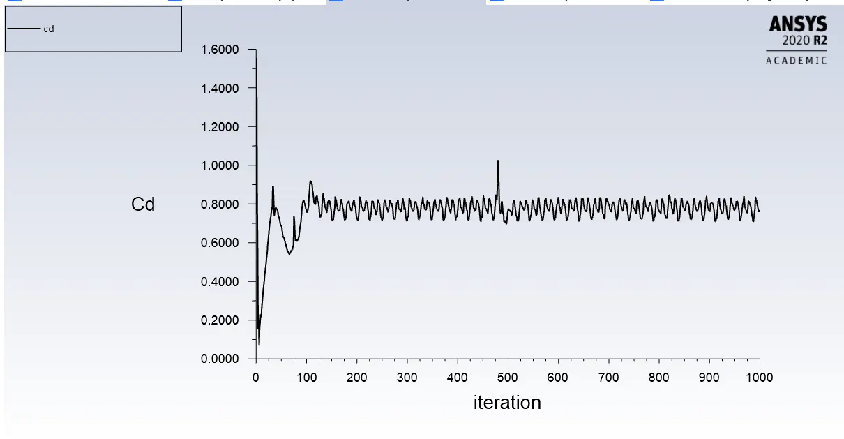
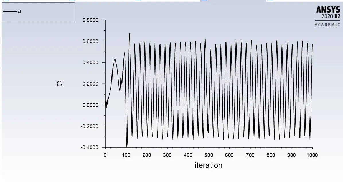
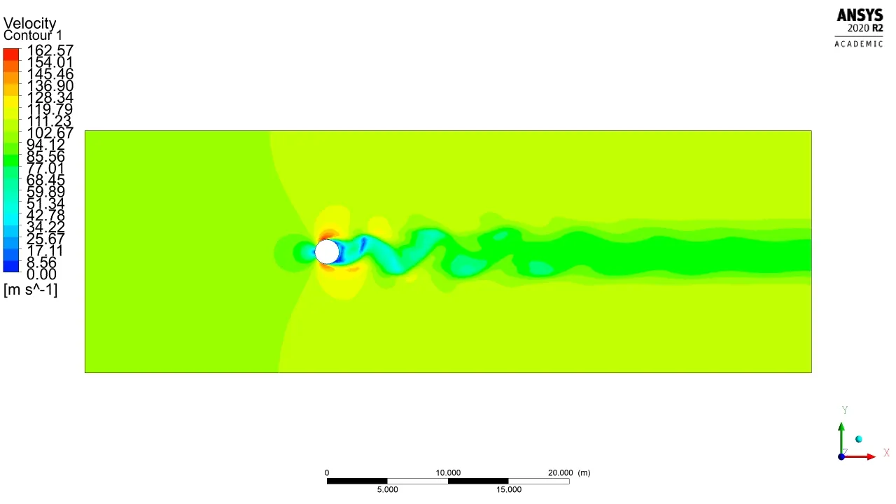
Reynolds Number: 10000

Viscosity: 0.02

Velocity: 100

Iterations: 1000

Residual plot:

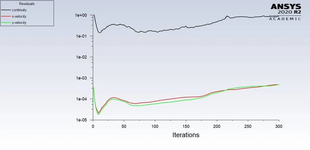
Monitor point velocity:

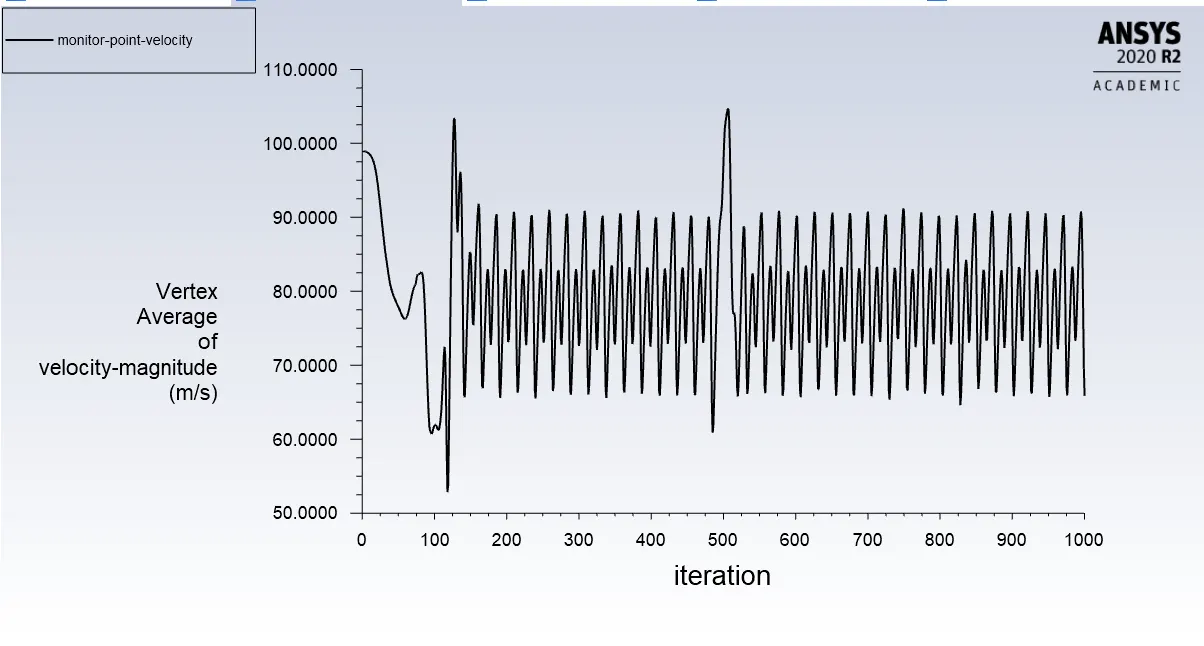
Drag Coefficient:

Lift coefficient:

Velocity contour:

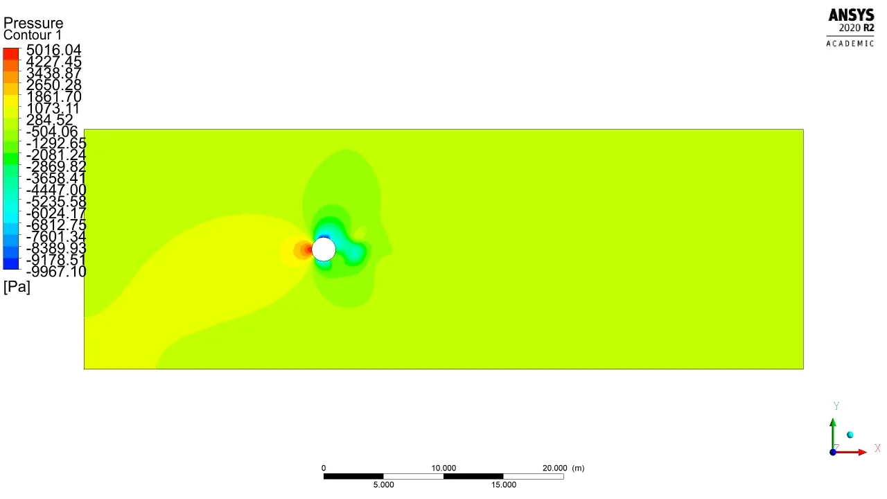
Case 5:

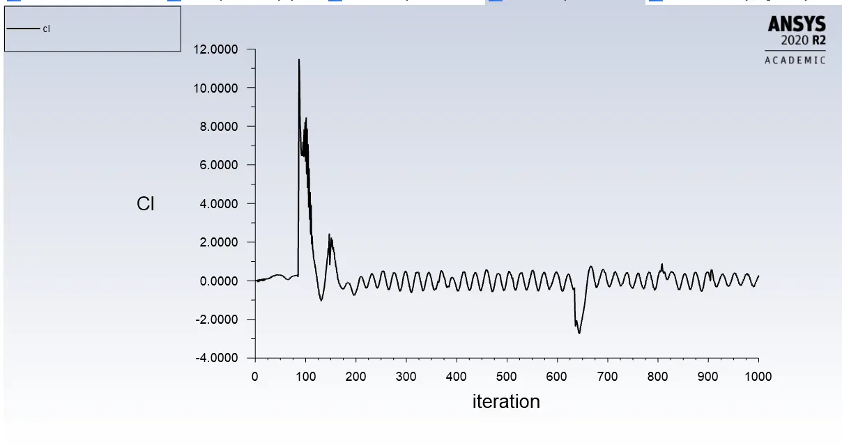
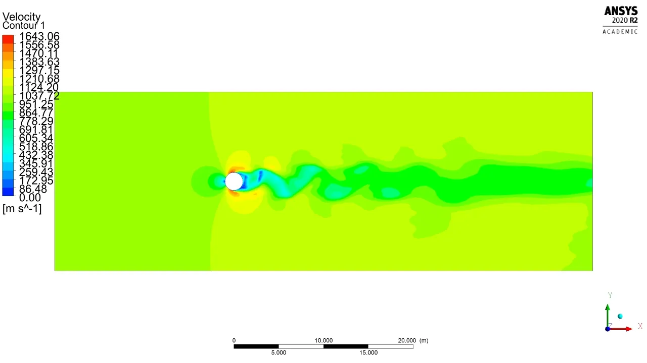
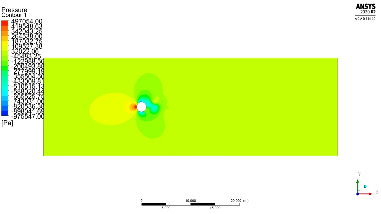
Reynolds Number: 100000

Viscosity:0.02

Velocity:1000

Iterations:1000

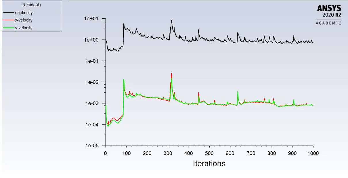
Residual plot:

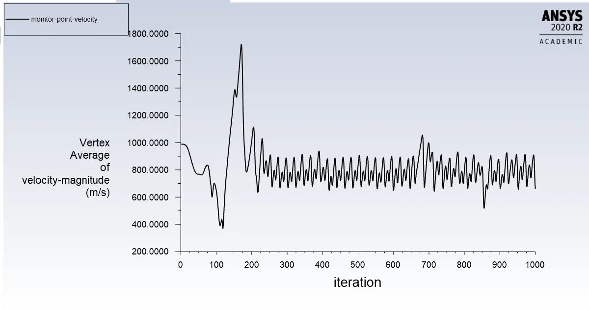
Monitor point velocity:

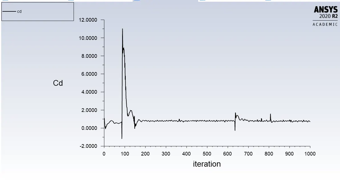
Drag Coefficient:

Lift coefficient:

Velocity contour:

Pressure contour:

Computed data are listed in the table.

Steady case Reynold's Number	Velocity @ Monitor Pt	Cd	Cl
10	0.043	3.32	-0.026
100	0.363	1.31	-0.113
1000	6.82	0.78	0.05
10000	70.83	0.77	0.32
100000	688.7	0.65	0.326

Reference Research Paper:- https://www.sciencedirect.com/science/article/pii/S0307904X08000243

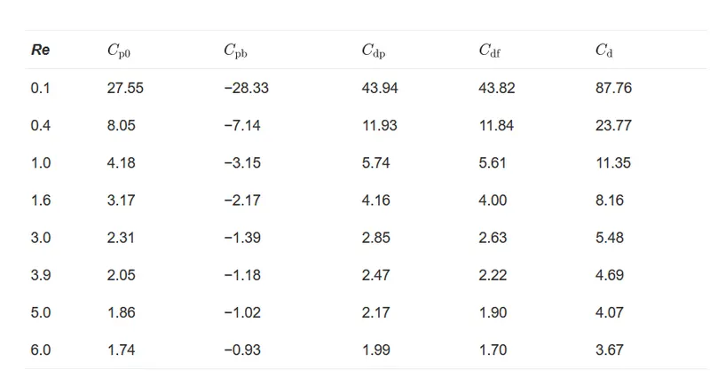
Conclusion : After inspecting the plots and contours provided above, with the increase in reynold number the drag-coefficient decreases and the lift-coefficient somewhat increases.

Material preffered for instability reduction:

1. Poruos Material
2. Spoiler plates (design dependant)
3. axial slits