Week 7 - Simulation of a 1D Super-sonic nozzle flow simulation using Macormack Method
clear all
close all
clc

%inputs
n=31;
x=linspace(0,3,n);
dx=x(2)-x(1);
gama=1.4;
nt=1000;% no. of time steps

%calculation of initial profile
rho= 1-0.3146*x;
T=1-0.2314*x;
v=(0.1 + 1.09*x).*T.^0.5;

% local sonic velocity
a1=(T).^0.5;

%area
a = 1 + 2.2*(x-1.5).^2;

% mass flow rate
m=(rho.*v).*a;
m_ini=m;

% times step
% (COURANT NUMBER)C=0.5
C=0.5;
%dt=0.0201;
dt1=C*(dx./(a1+v));
dt=min(dt1);

% defining time varying variables
t_avg=16;
rho_t_avg=ones(1,nt);
v_t_avg=ones(1,nt);
T_t_avg=ones(1,nt);
M_t_avg=ones(1,nt);
P_t_avg=ones(1,nt);

% defining the time varying flow-field derivatives
drhodt_t_avg=ones(1,nt);
dvdt_t_avg=ones(1,nt);
dTdt_t_avg=ones(1,nt);


% outer time loop
for k=1:nt

    rho_old=rho;
    v_old=v;
    T_old=T;
    % predictor method
    for j=2:n-1

        dvdxp=(v(j+1)-v(j))/dx;
        drhodxp=(rho(j+1)-rho(j))/dx;
        dTdxp=(T(j+1)-T(j))/dx;
        dlogadxp=(log(a(j+1)) - log(a(j)))/dx;

        % CONTINUITY EQUATION
        drhodt_p(j)= -rho(j)*dvdxp -rho(j)*v(j)*dlogadxp -v(j)*drhodxp;

        % MOMENTUM EQUATION
        dvdt_p(j)= -v(j)*dvdxp -(1/gama)*(dTdxp + ((T(j)*drhodxp)/(rho(j))));

        % ENERGY EQUATION
        dTdt_p(j)= -v(j)*dTdxp -(gama-1)*T(j)*(dvdxp + v(j)*dlogadxp);

        % solution update
        rho(j) = rho_old(j) + drhodt_p(j)*dt;
        v(j) = v_old(j) + dvdt_p(j)*dt;
        T(j) = T_old(j) + dTdt_p(j)*dt;
    end
    % corrector method
    for f=2:n-1

        dvdx = (v(f)-v(f-1))/dx;
        drhodx = (rho(f)-rho(f-1))/dx;
        dTdx = (T(f)-T(f-1))/dx;
        dlogadx = (log(a(f))-log(a(f-1)))/dx;

        % CONTINUITY EQUATION
        drhodt_c(f)= -rho(f)*dvdx -rho(f)*v(f)*dlogadx -v(f)*drhodx;

        % MOMENTUM EQUATION
        dvdt_c(f)= -v(f)*dvdx -(1/gama)*(dTdx + ((T(f)*drhodx)/(rho(f))));

        % ENERGY EQUATION
        dTdt_c(f)= -v(f)*dTdx -(gama-1)*T(f)*(dvdx + v(f)*dlogadx);
    end
    % compute the average time derivative
    drhodt = 0.5*(drhodt_p + drhodt_c);
    dvdt = 0.5*(dvdt_p + dvdt_c);
    dTdt = 0.5*(dTdt_p + dTdt_c);

    % capture time varying flow-dield derivative
    drhodt_t_avg(k)=drhodt(t_avg);
    dvdt_t_avg(k)=dvdt(t_avg);
    dTdt_t_avg(k)=dTdt(t_avg);

    %final solution update
    for i=2:n-1
    rho(i) = rho_old(i) + drhodt(i)*dt;
    v(i) = v_old(i) + dvdt(i)*dt;
    T(i) = T_old(i) + dTdt(i)*dt;
    end

    %apply the boundary condition
    % inlet
    v(1) = 2*v(2) - v(3);
    %outlet
    v(n) = 2*v(n-1) - v(n-2);
    rho(n) = 2*rho(n-1) - rho(n-2);
    T(n) = 2*T(n-1) - T(n-2);

    % mass flow rate
    m=(rho.*v).*a;
    % capturing the mass flow in the nozzle at different time step
    if k==1
        m_1=m;
    end
    if k==50
        m_50=m;
    end
    if k==100
        m_100=m;
    end
    if k==150
        m_150=m;
    end
    if k==200
        m_200=m;
    end
    if k==700
        m_700=m;
    end

    % Mach number (M)
    M = v./(T.^0.5);

    % Non-dimensional Pressure
    P = rho.*T;

    % capturing time wise variation of pressure and mach number at the nozzle throat
    M_t_avg(k)=M(t_avg);
    P_t_avg(k)=P(t_avg);

    figure(1)
    subplot(1,3,1)
    plot(x,rho,'b')
    title(sprintf('time step=%d',k))
    subplot(1,3,2)
    plot(x,v,'r')
    title(sprintf('time step=%d',k))
    subplot(1,3,3)
    plot(x,T,'g')
    title(sprintf('time step=%d',k))

    % capturing time wise variation of flow properties at the nozzle throat
    rho_t_avg(k)=rho(t_avg);
    v_t_avg(k)=v(t_avg);
    T_t_avg(k)=T(t_avg);

    % Update the value of time step
    a1=(T).^0.5;
    dt1=C*(dx./(a1+v));
    dt=min(dt1);
end
% steady-state flow-field distributions along nozzle
figure(2)
plot(x,rho,'b')
title('STEADY-STATE FLOW-FIELD DISTRIBUTION NON-DIMENSIONAL DENSITY')
xlabel('x-axis')
ylabel('NON-DIMENSIONAL DENSITY rho/rho0')

figure(3)
plot(x,v,'r')
title('STEADY-STATE FLOW-FIELD DISTRIBUTION NON-DIMENSIONAL VELOCITY')
xlabel('x-axis')
ylabel('NON-DIMENSIONAL VELOCITY V/a')

figure(4)
plot(x,T,'g')
title('STEADY-STATE FLOW-FIELD DISTRIBUTION NON-DIMENSIONAL TEMPERATURE')
xlabel('x-axis')
ylabel('NON-DIMENSIONAL TEMPERATURE T/T0')

figure(5)
plot(x,M,'k')
title('STEADY-STATE FLOW-FIELD DISTRIBUTION MACH NUMBER')
xlabel('x-axis')
ylabel('MACH NUMBER (local velocity/local sonic velocity)')

figure(6)
plot(x,P,'k')
title('STEADY-STATE FLOW-FIELD DISTRIBUTION NON-DIMENSIONAL PRESSURE')
xlabel('x-axis')
ylabel('NON-DIMENSIONAL PRESSURE P/P0')

% ploting the flow-field variation at 15th grid point w.r.t time step
figure(7)
plot(rho_t_avg)
title('Time-wise variation of the primative variables at the nozzle throat')
xlabel('time-axis')
ylabel('NON-DIMENSIONAL DENSITY rho/rho0')

figure(8)
plot(v_t_avg)
title('Time-wise variation of the primative variables at the nozzle throat')
xlabel('time-axis')
ylabel('NON-DIMENSIONAL VELOCITY V/a')

figure(9)
plot(T_t_avg)
title('Time-wise variation of the primative variables at the nozzle throat')
xlabel('time-axis')
ylabel('NON-DIMENSIONAL TEMPERATURE T/T0')

figure(10)
plot(M_t_avg)
title('Time-wise variation of MACH NUMBER AT THROAT SECTION')
xlabel('time-axis')
ylabel('MACH NUMBER')

figure(11)
plot(P_t_avg)
title('Time-wise variation of NON-DIMENSIONAL PRESSURE AT THROAT SECTION')
xlabel('time-axis')
ylabel('NON-DIMENSIONAL PRESSURE P/P0')

% ploting the time derivatives as a function of time
figure(12)
plot(drhodt_t_avg,'r')
title('Time-wise variation of the flow-field derivative at the nozzle throat')
xlabel('time-axis')
ylabel('NON-DIMENSIONAL DENSITY DERIVATIVE')

figure(13)
plot(dvdt_t_avg,'b')
title('Time-wise variation of the flow-field derivative at the nozzle throat')
xlabel('time-axis')
ylabel('NON-DIMENSIONAL VELOCITY DERIVATIVE')

figure(14)
plot(dTdt_t_avg,'k')
title('Time-wise variation of the flow-field derivative at the nozzle throat')
xlabel('time-axis')
ylabel('NON-DIMENSIONAL TEMPERATURE DERIVATIVE')

figure(15)
plot(m_ini,'b')
hold on
plot(m_50,'r')
hold on
plot(m_100,'g')
hold on
plot(m_150,'b')
hold on
plot(m_200,'r')
hold on
plot(m_700,'k')
hold on
legend('0*dt','50*dt','100*dt','150*dt','200*dt','700*dt')
title('TIME WISE VARIATION OF NON-DIMENSIONAL MASS FLOW RATE DISTRIBUTION IN THE NOZZLE')
xlabel('x-axis')
ylabel('NON-DIMENSIONAL MASS FLOW RATE ')
clear all
close all
clc

%inputs
n=31;
x=linspace(0,3,n);
dx=x(2)-x(1);
gama=1.4;
nt=1000;

%area
a = 1 + 2.2*(x-1.5).^2;

%initial conditions
rho=ones(1,length(x));
T=ones(1,length(x));
for i=7:16
    rho(1,i) = 1-0.366*(x(1,i)-0.5);
    T(1,i) = 1-0.167*(x(1,i)-0.5);
end
for i=16:31
    rho(1,i) = 0.634-0.3879*(x(1,i)-1.5);
    T(1,i) = 0.833-0.3507*(x(1,i)-1.5);
end

% local sonic velocity
a1=(T).^0.5;

% initital velocity vector
v = 0.59./(rho.*a);

% mass flow rate
m=(rho.*v).*a;
m_ini=m;

% initial solution vector
u1 = rho.*a;
u2 = (rho.*a).*v;
u3 = (rho.*a).*( T/(gama-1) + (v.^2)*(gama/2) );

% times step
% COURANT NUMBER
C=1.1;
%dt=0.0467;
dt1=C*(dx./(a1+v));
dt=min(dt1);

% defining time varying variables
t_avg=16;
rho_t_avg=ones(1,nt);
v_t_avg=ones(1,nt);
T_t_avg=ones(1,nt);
M_t_avg=ones(1,nt);
P_t_avg=ones(1,nt);

% defining the time varying flow-field derivatives
drhodt_t_avg=ones(1,nt);
dvdt_t_avg=ones(1,nt);
dTdt_t_avg=ones(1,nt);

%time loop
for k=1:nt
    % COPY OF THE PRIMITIVE VARIABLES
    u1_old=u1;
    u2_old=u2;
    u3_old=u3;

    % PREDICTOR METHOD
    for j=2:n-1
        % FLUX TERMS AND SOURCE TERMS
        f1 = u2;
        f2 = ((u2.^2)./u1) + ((gama-1)/gama)*(u3 - (gama*0.5)*((u2.^2)./u1));
        f3 = gama*((u2.*u3)./u1) - (gama*(gama-1)*0.5)*((u2.^3)./(u1.^2));
        J2 = (((gama-1)/gama)*(u3 - (gama/2)*((u2.^2)./(u1))));
        dlogadx = (log(a(j+1)) - log(a(j)))/dx;

        % CONTINUITY EQUATION
        du1dt_p(j) = -(f1(j+1) - f1(j))/dx;

        % MOMENTUM EQUATION
        du2dt_p(j) = -((f2(j+1) - f2(j))/dx) + J2(j)*dlogadx;

        % ENERGY EQUATION
        du3dt_p(j) = -(f3(j+1) - f3(j))/dx;

        % UPDATING THE SOLUTION VECTOR
        u1(j) = u1_old(j) + du1dt_p(j)*dt;
        u2(j) = u2_old(j) + du2dt_p(j)*dt;
        u3(j) = u3_old(j) + du3dt_p(j)*dt;
    end
    % CORRECTOR METHOD
    for j=2:n-1

        % UPDATING THE FLUX TERMS AND THE SOURCE TERMS
        f1 = u2;
        f2 = ((u2.^2)./u1) + ((gama-1)/gama)*(u3 - (gama/2)*((u2.^2)./u1));
        f3 = gama*((u2.*u3)./u1) - (gama*(gama-1)*0.5)*((u2.^3)./(u1.^2));
        J2 = (((gama-1)/gama)*(u3 - (gama/2)*((u2.^2)./(u1))));
        dlogadx = (log(a(j)) - log(a(j-1)))/dx;

        % CONTINUITY EQUATION
        du1dt_c(j) = -(f1(j) - f1(j-1))/dx;

        % MOMENTUM EQUATION
        du2dt_c(j) = -((f2(j) - f2(j-1))/dx) + J2(j)*dlogadx;

        % ENERGY EQUATION
        du3dt_c(j) = -(f3(j) - f3(j-1))/dx;
    end
    % EVALUATE THE AVERAGE DERIVATIVE
    du1dt_av = 0.5*(du1dt_c + du1dt_p);
    du2dt_av = 0.5*(du2dt_c + du2dt_p);
    du3dt_av = 0.5*(du3dt_c + du3dt_p);

    % capture time varying flow-dield derivative
    drhodt_t_avg(k)=du1dt_av(t_avg);
    dvdt_t_avg(k)=du2dt_av(t_avg);
    dTdt_t_avg(k)=du3dt_av(t_avg);

    % updating the solution vector
    for i=2:n-1
        u1(i) = u1_old(i) + du1dt_av(i)*dt;
        u2(i) = u2_old(i) + du2dt_av(i)*dt;
        u3(i) = u3_old(i) + du3dt_av(i)*dt;
    end

    %apply the boundary condition
    % inlet
    u2(1) = 2*u2(2) - u2(3);
    %outlet
    u1(n) = 2*u1(n-1) - u1(n-2);
    u2(n) = 2*u2(n-1) - u2(n-2);
    u3(n) = 2*u3(n-1) - u3(n-2);

    % define the dependent variables
    rho=u1./a;
    v=u2./u1;
    T=(gama-1)*(u3./u1 - (gama/2)*(u2./u1).^2);

    % mass flow rate
    m=(rho.*v).*a;
    % capturing the mass flow in the nozzle at different time step
    if k==1
        m_1=m;
    end
    if k==50
        m_50=m;
    end
    if k==100
        m_100=m;
    end
    if k==150
        m_150=m;
    end
    if k==200
        m_200=m;
    end
    if k==700
        m_700=m;
    end

    % Mach number (M)
    M = v./(T.^0.5);

    % Non-dimensional Pressure
    P = rho.*T;

    % capturing time wise variation of pressure and mach number at the nozzle throat
    M_t_avg(k)=M(t_avg);
    P_t_avg(k)=P(t_avg);


    % update the values for dt
    a1=(T).^0.5; % a1 = local sonic-velocity
    dt1=C*(dx./(a1 + v));
    dt=min(dt1);

    % capturing time wise variation of flow properties at the nozzle throat
    rho_t_avg(k)=rho(t_avg);
    v_t_avg(k)=v(t_avg);
    T_t_avg(k)=T(t_avg);

    % steady-state variation of floe-field properties
    figure(1)
    subplot(1,3,1)
    plot(x,rho,'b')
    title(sprintf('time step=%d',k))
    subplot(1,3,2)
    plot(x,v,'r')
    title(sprintf('time step=%d',k))
    subplot(1,3,3)
    plot(x,T,'g')
    title(sprintf('time step=%d',k))

end

% UPDATING THE FINAL VALUES
rho=u1./a;
v=u2./u1;
T=(gama-1)*(u3./u1 - (gama/2)*(u2./u1).^2);

% steady-state flow-field distributions along nozzle
figure(2)
plot(x,rho,'b')
title('STEADY-STATE FLOW-FIELD DISTRIBUTION NON-DIMENSIONAL DENSITY')
xlabel('x-axis')
ylabel('NON-DIMENSIONAL DENSITY rho/rho0')

figure(3)
plot(x,v,'r')
title('STEADY-STATE FLOW-FIELD DISTRIBUTION NON-DIMENSIONAL VELOCITY')
xlabel('x-axis')
ylabel('NON-DIMENSIONAL VELOCITY V/a')

figure(4)
plot(x,T,'g')
title('STEADY-STATE FLOW-FIELD DISTRIBUTION NON-DIMENSIONAL TEMPERATURE')
xlabel('x-axis')
ylabel('NON-DIMENSIONAL TEMPERATURE T/T0')

figure(5)
plot(x,M,'k')
title('STEADY-STATE FLOW-FIELD DISTRIBUTION MACH NUMBER')
xlabel('x-axis')
ylabel('MACH NUMBER (local velocity/local sonic velocity)')

figure(6)
plot(x,P,'k')
title('STEADY-STATE FLOW-FIELD DISTRIBUTION NON-DIMENSIONAL PRESSURE')
xlabel('x-axis')
ylabel('NON-DIMENSIONAL PRESSURE P/P0')

% ploting the flow-field variation at 15th grid point w.r.t time step
figure(7)
plot(rho_t_avg)
title('Time-wise variation of the primative variables')
xlabel('time-axis')
ylabel('NON-DIMENSIONAL DENSITY rho/rho0')

figure(8)
plot(v_t_avg)
title('Time-wise variation of the primative variables')
xlabel('time-axis')
ylabel('NON-DIMENSIONAL VELOCITY V/a')

figure(9)
plot(T_t_avg)
title('Time-wise variation of the primative variables')
xlabel('time-axis')
ylabel('NON-DIMENSIONAL TEMPERATURE T/T0')

% ploting the time derivatives as a function of time
figure(10)
plot(drhodt_t_avg,'r')
title('Time-wise variation of the flow-field derivative')
xlabel('time-axis')
ylabel('NON-DIMENSIONAL DENSITY rho/rho0')

figure(11)
plot(dvdt_t_avg,'b')
title('Time-wise variation of the flow-field derivative')
xlabel('time-axis')
ylabel('NON-DIMENSIONAL VELOCITY V/a')

figure(12)
plot(dTdt_t_avg,'k')
title('Time-wise variation of the flow-field derivative')
xlabel('time-axis')
ylabel('NON-DIMENSIONAL TEMPERATURE T/T0')

figure(13)
plot(m_ini,'b')
hold on
plot(m_50,'r')
hold on
plot(m_100,'g')
hold on
plot(m_150,'b')
hold on
plot(m_200,'r')
hold on
plot(m_700,'k')
hold on
legend('0*dt','50*dt','100*dt','150*dt','200*dt','700*dt')
title('TIME WISE VARIATION OF NON-DIMENSIONAL MASS FLOW RATE DISTRIBUTION IN THE NOZZLE')
xlabel('x-axis')
ylabel('NON-DIMENSIONAL MASS FLOW RATE ')
ISENTROPIC QUASI 1-DIMENSIONAL SUBSONIC/SUPERSONIC NOZZLE FLOW (CONVERGENT-DIVERGENT NOZZLE)
--> We have a conergent-divergent nozzle whos inlet is connected to a reservoir with fluid at a particular temperature(T0), pressure(p0), density(ρ0) with a large area(tending to infinity) and very low velocity.
PHYSICAL PROBLEM:--
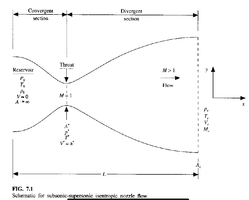
The above schematic diagram represents the physical situation of the convergent-divergent nozzle flow.(The refference of this diagram is taken from John Anderson Computational Fluid Dynamics-McGraw-Hill (1995) )
We consider an isentropic flow through a convergent-divergent nozzle. The flow comes from a reservoir where (T0,p0,ρ0) are the stagnation values. The cross-sectional area is very large (A--->∞) theoretically and hence velocity is very small(v--->0). The flow field expands isentropically to the supersonic speeds at the nozzle exit. The flow locally is sub-sonic at the convergent section,sonic at the throat (minimum area) and attains super-sonic speeds at the exit. At throat velovity "v" is equal to the local speed of sound at the throat. At the throat section we have (v=v*=a*) similarly the sonic flow values at the throat section we have pressure (p*), temperature (T*) and density(ρ*) . Area of sonic throat(A*).
QUASI-1D ASSUMPTION--> We assume at a given cross section the flow properties are uniform across this section although in reality the flow field is 2 dimensional (flow properties vary in 2 dimensional space) but we assume that the flow properties vary only along "x" direction and at a given cross-section the flow properties are constant. Such flows are defined as the quasi 1-D flow.
GOVERNING FLOW EQUATIONS [CONTINUITY, MOMENTUM, ENERGY] FOR QUASI 1-D ISENTROPIC NOZZLE FLOW -->
-->
NON-CONSERVATION FORM --> [1]. Mass conservation equation --> ∂(ρ)/∂t + ρ( ∂v/∂x ) + v( ∂ρ/∂x ) + ρv( ∂ln(a)/∂x ) = 0
[2]. Momentum conservation equation --> ρ( ∂v/∂t ) + ρv( ∂v/∂x ) = -∂p/∂x
(Equation of state) P=ρRT ==> (applying chain rule) ∂v/∂t = -v(∂v/∂x) - R(∂T/∂x + (T/ρ)(∂ρ/∂x))
[3]. Energy conservation equation --> ρ(cv)( ∂T/∂t ) + ρv(cv)( ∂T/∂x ) = -p( ∂v/∂x ) - pv( ∂ln(a)/∂x )
(Equation of state) P=ρRT ==> ρ(cv)( ∂T/∂t ) + ρv(cv)( ∂T/∂x ) = -ρRT[∂v/∂x + v(∂ln(a)/∂x)]
CONSERVATION FORM --> [1]. Mass conservation equation --> ∂( ρa )/∂t + ∂( ρav )/∂x = 0
[2]. Momentum conservation equation --> ∂( ρav )/∂t + ∂( ρav^2 + pa )/∂x = p(∂a/∂x)
[3]. Energy conservation equation --> ∂[ ρa(e + (v^2)/2) ]/∂t + ∂[ ρav(e + (v^2)/2)) + pav ]/∂x = 0
THE NON-DIMENSIONAL VARIABLES --> [1]. Non-dimensional temperature = T/T0
[2]. Non-dimensional density => ρ/ρ0 = ρ'
[3]. Non-dimensional pressure => p/p0 = p'
[4]. Non-dimensional length => x' = x/L
[5]. Non-dimensional sonic-velocity => a' = a/a0 = (γRT)^0.5/(γR(T0))^0.5 = (T/T0)^0.5 = (T')^0.5
[6]. Non-dimensional velocity => v' = v/a0
[7]. Non-dimensional time => t' = t/t0
[8]. Non-dimensional Area => a' = a/a*
[9]. Non-dimensional internal energy => e' = e/e0 = cv(T)/cv(T0) = T/T0 = T'
--> Mach-number ---- M = v/(T^0.5)
--> For a calorically perfect gas ---- e=cv(T)
--> Equation of state ------- p=ρRT
--> p'=(RρT)/(Rρ0T0)= (ρT)/(ρ0T0)=ρ'T'
--> Mach number is already a non-dimensional parameter and is defined by local velocity divided by local speed of sound wave.
--> a0=stagnation sonic velocity (at the reservoir)
NON-DIMENSIONAL NON-CONSERVATION GOVERNING EQUATION-->
[1]. Continuity Equation ----> ∂ρ'/∂t' + ρ'( ∂v'/∂x' ) + v'( ∂ρ'/∂x' ) + ρ'v'( ∂ln(a')/∂x' ) = 0
[2]. Momentum conservation equation --> ( ∂v'/∂t' ) = -v'( ∂v'/∂x' ) -(1/γ)(∂T'/∂x' + (T'/ρ')(∂ρ'/∂x'))
[3]. Energy conservation equation --> ( ∂T'/∂t' ) = -v'( ∂T'/∂x' ) -(γ-1)T'( ∂v'/∂x' + v'(∂ln(a')/∂x') )
NON-DIMENSIONAL CONSERVATION GOVERNING EQUATION-->
[1]. Mass conservation equation --> ∂( ρ'a' )/∂t' + ∂( ρ'a'v' )/∂x' = 0
[2]. Momentum conservation equation --> ∂( ρ'a'v' )/∂t' + ∂( ρ'a'v'^2 + (1/γ)p'a' )/∂x' = (1/γ)p'(∂a'/∂x')
[3]. Energy conservation equation --> ∂[ ρ'a'(T'/γ-1 + (γ/2)(v'^2)/2) ]/∂t' + ∂[ ρ'a'v'(T'/γ-1 + (γ/2)(v'^2)/2)) + p'a'v' ]/∂x' = 0
MACCORMACKS METHOD FOR NON-CONSERVATION GOVERNING EQUATION FORM--->
--> calculation of the time step "dt"
For a linear hyperbolic equation there exists a stability constraint on the system. A simple stability analysis gives us condition on courant number.
dt=C(dx/(a+v))
C<=1
The above inequality is the constriant for stability of linear hyperbolic PDE.
note:-- The above is not derived for non-linear hyperbolic PDE. But it serves as a guidance for our present analysis. It simply states that "dt" should be less than or at best equal to the time required for sound wave to travel from 1 grid point to another.
--> Boundary conditions
At inflow boundary we allow 1 dependent variable ('v' velocity) to float with the solution and allocate fixed values to 2 dependent variables(density (rho) and temperature(T)).
This is mainly because 1 characteristic is propagating out of the domain and the other is moving in to the domain relative to the initial point at the sonic speed, and also the streamline is propagating into the domain.
Using the same assertion we can say at the outlet both the characteristic and the streamline are flowing out of the domain and therefore we have to allow all the dependent variable to float with the solution.
--> Results of non-conservation form
1. STEADY-STATE FLOW-PROPERTIES INSIDE THE NOZZLE
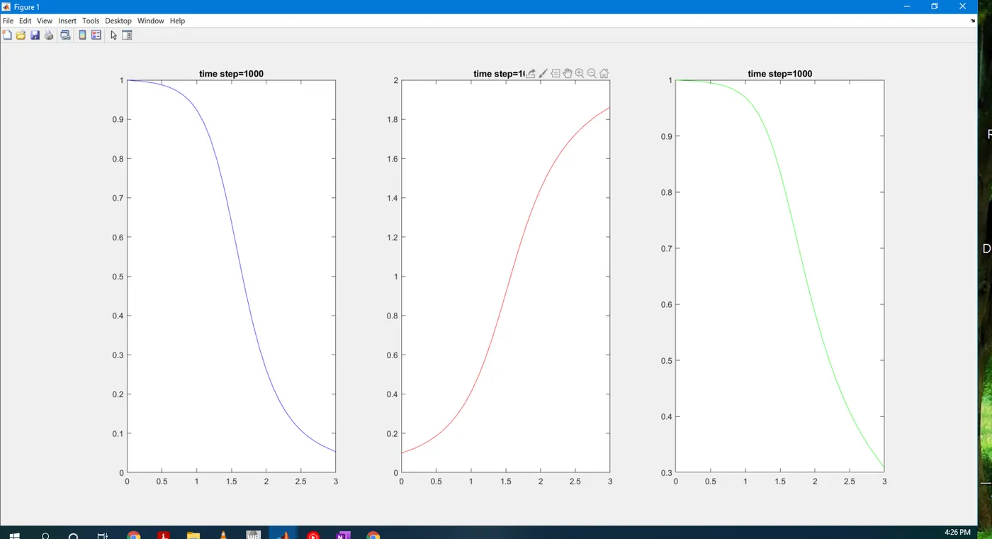
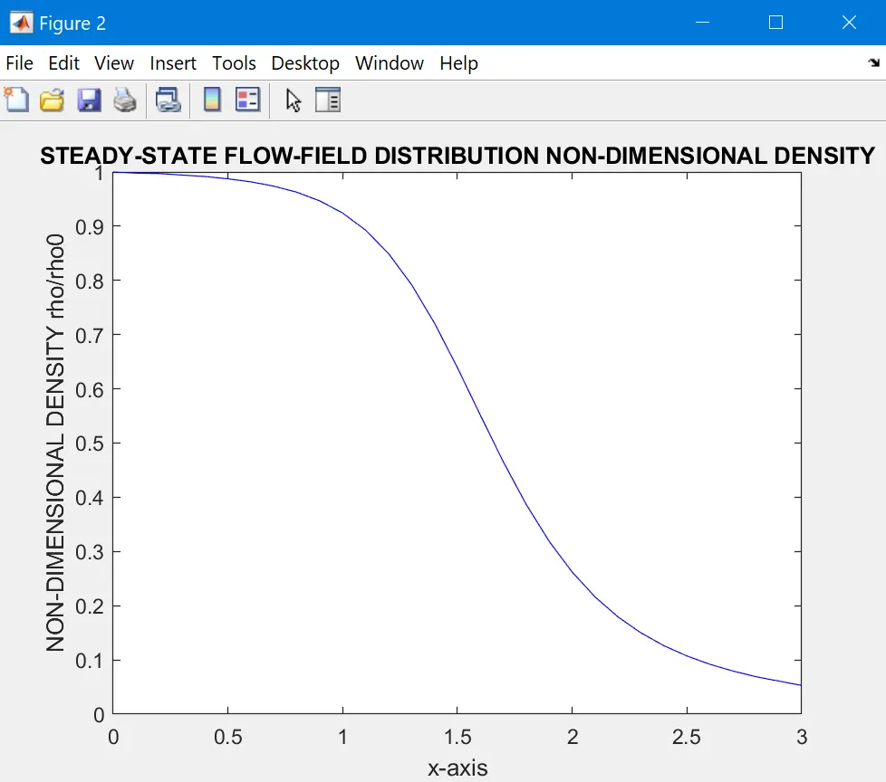
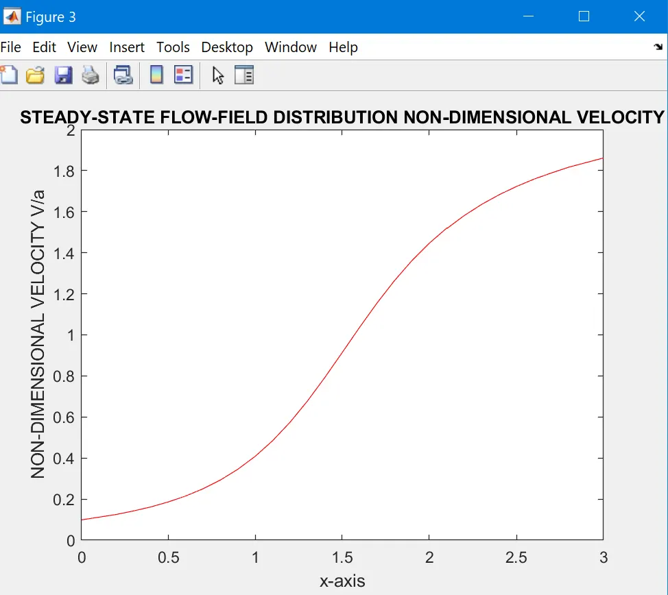
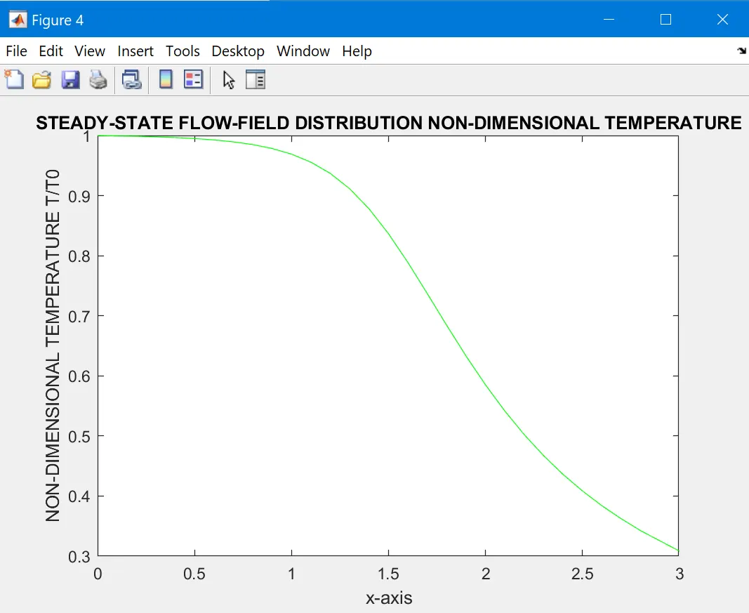
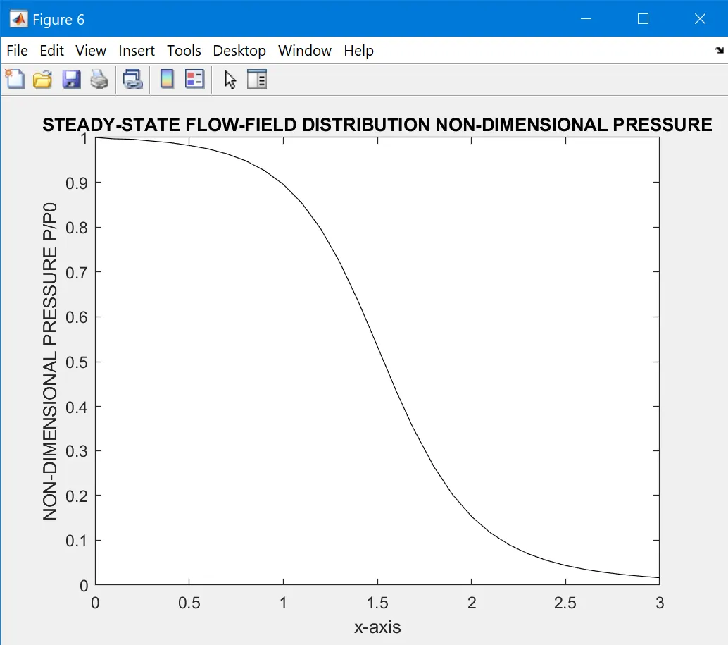
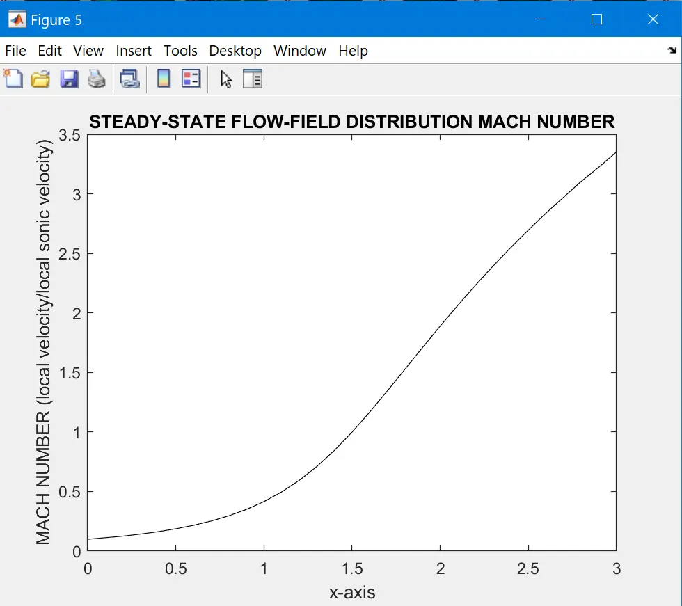
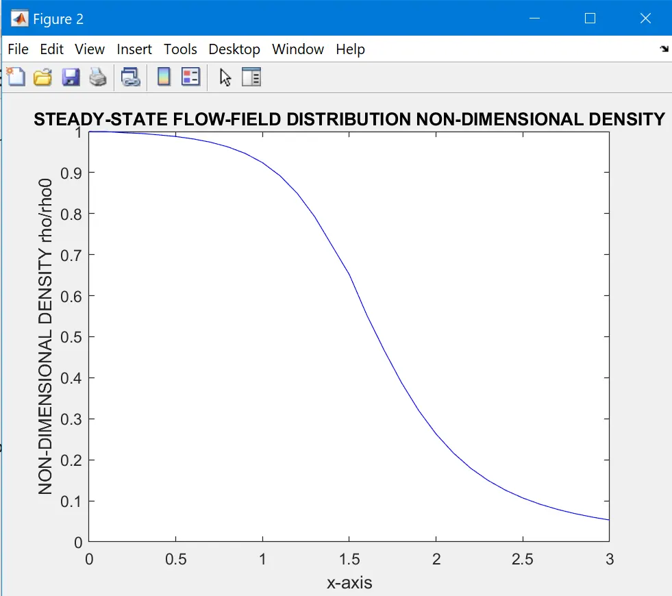
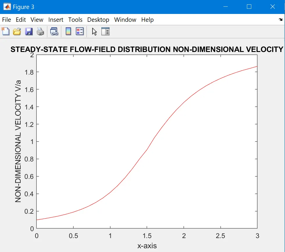
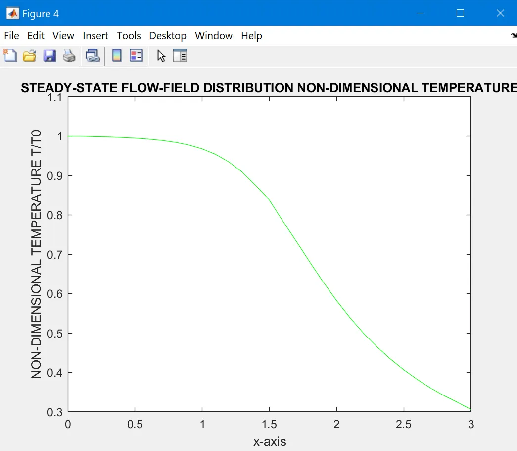
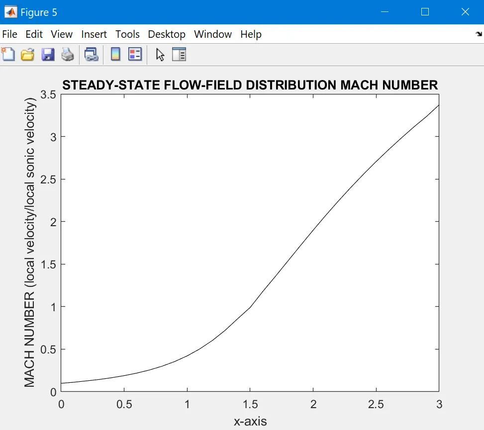
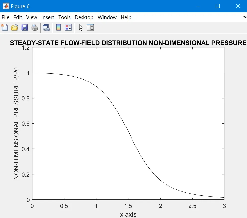
--> The above graphs demonstrate the steady-state distribution of the primative variables inside the nozzle. All the variables are in the non-dimensional form. Y-axis represents the non-dimensional flow variable and the X-axis represents the non-dimensional length along the nozzle.
-->We can see that steady-state for all practical purposes is achieved at the 500 time steps. Within the graphical accuracy the analytical results agree to a large extent with the numerical results.
2. TIME WISE VARIATION OF FLOW-PROPERTIES INSIDE THE NOZZLE AT A PARTICULAR GRID POINT
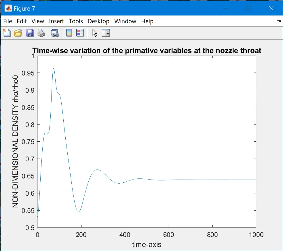
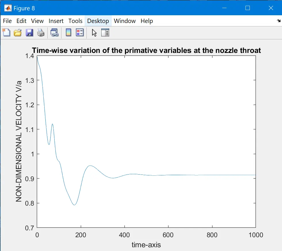
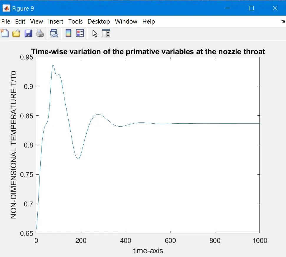
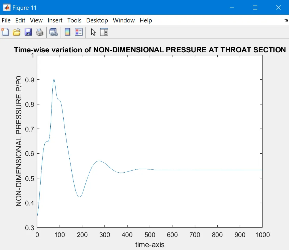
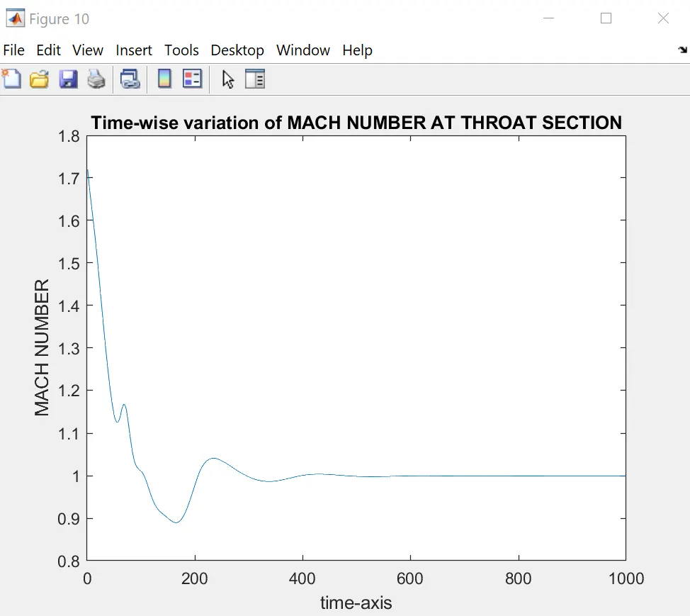
--> The above graphs illustrate the flow-field variables at the throat section along the time steps or time axis. We note that at the initial time largest changes takes place and final steady-state values is approached asymptotically. Rapid changes occur at the initial time and there is a strong potential of change at initial time.
3. TIME WISE VARIATION OF FLOW-PROPERTY DERIVATIVES INSIDE THE NOZZLE AT THROAT SECTION
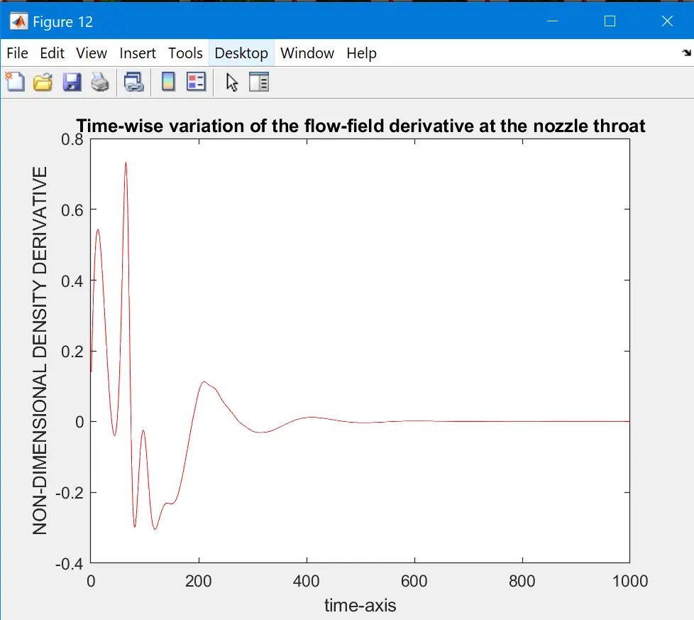
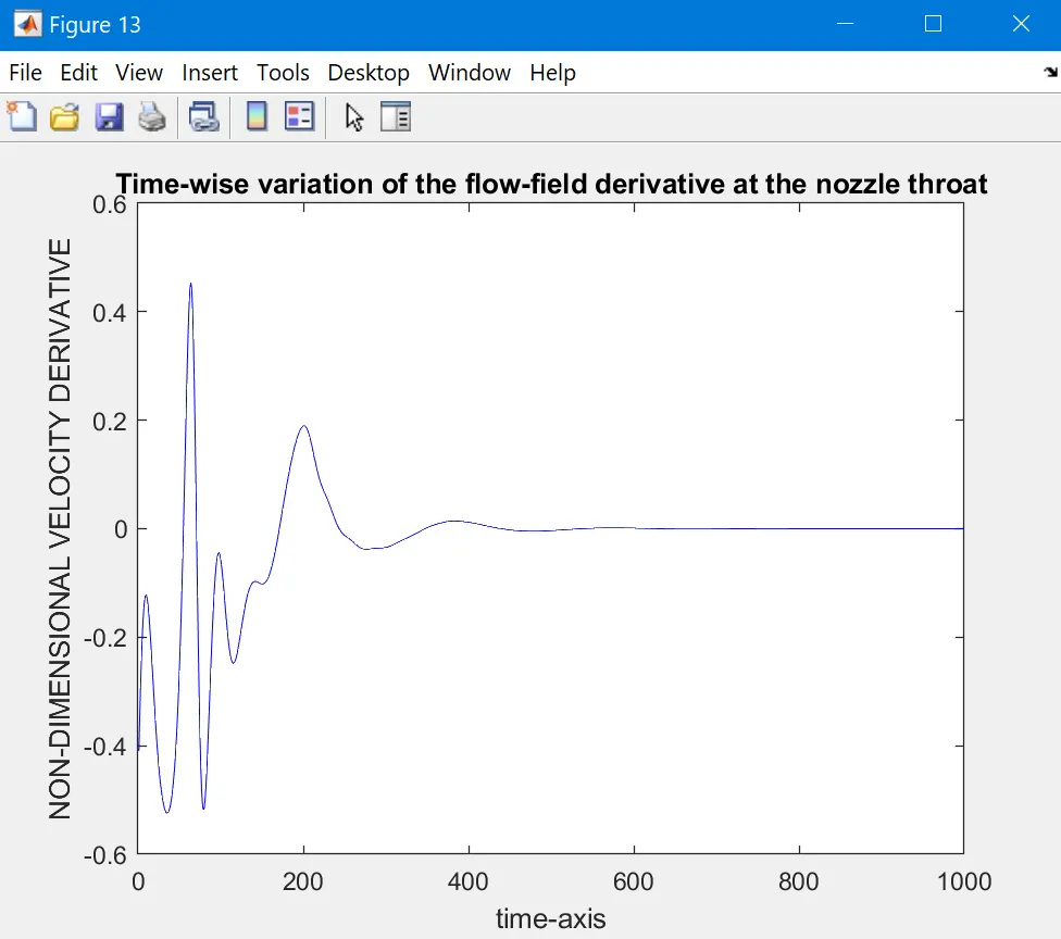
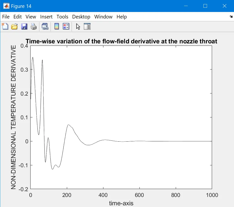
--> These are the average time derivatives calculated at the nozzle throat w.r.t the time step. We are examining variation in the time derivatives (density temperature velocity) with respect to time.
1. At early time steps, the time derivatives are large and they oscillate in value. There are unsteady expansion and compression waves propagating during the transient process.
2. At later time steps, the time derivatives rapidly grow small over the span of 1000 time steps. Theoritacally at steady-state the time derivatives should go to zero value. Numerically these values never go to zero, but attain very small values close to zero and practically steady-state is achieved.
4. TIME WISE VARIATION OF MASS FLOW RATE DISTRIBUTION AT THROAT SECTION & STEADY-STATE DISTRIBUTION
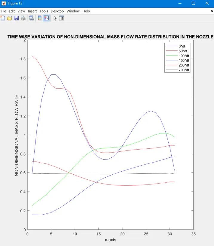
--> 6 different curves are shown ,each for a different time during the course of time-marching procedure. Mass flow rate variation is shown.
--> After 50 time steps the mass flow distribution through the nozzle has changed considerably. The mass flow variation is simply flopping around inside the nozzle due to the transient variation of the flow field variables. However after 200 time steps the mass flow is begining to settle down and after 700 time steps mass flow is straight horizontal line. This says that mass flow has converged to steady-state value constant throughtout the nozzle.This also agrees to ρAV=constant
--> RESULTS OF CONSREVATION FORM
--> We use a generic form of the variables.
[1]. u1=ρ'A'
[2]. u2=ρ'A'V'
[3]. u3=ρ'A'[T'/γ-1 + (γ/2)V'^2]
[4]. F1=ρ'A'V'
[5]. F2=ρ'A'V'^2 + 1/γ(P'A')
[6]. F3=ρ'A'[T'/γ-1 + (γ/2)V'^2] + P'A'V'
[7]. J2=(1/γ)P'(dA'/dx')
--> We define the solution vector ,source terms and the flux terms and solve the conservation PDE that is discussed above.
--> The dependent variables which occur in the governing PDE are u1,u2 and u3 so all the flux and source terms should be represented as a function of these variables only.If we use the primitive variables we might get unstable results. This is also known as the pure form of the conservation equations.
--> Boundary conditions and the time step calculation is almost the same as that of the non-conservation form ,but we use a slightly more accurate initial conditions in terms of the closeness to the actual results. We want to take initial condition close to the actual results.
Principally to take advantage of the fact that u2 is the local mass flow rate and that we should choose our initial condition intelligiently, we take a constant mass flow rate (0.59). Mass flow distribution originally choosen to be a constant is no longer a constant after the first time step. Largest changes over the first time step takes place at the end of the nozzle.
--> A quick comparison of the results from the non-conservation and conservation reveals that both show little material difference and for all practical purposes both forms give same results. However in problems related to shock capturing conservation form is more suitable.
2. TIME WISE VARIATION OF MASS FLOW RATE DISTRIBUTION AT THROAT SECTION & STEADY-STATE DISTRIBUTION
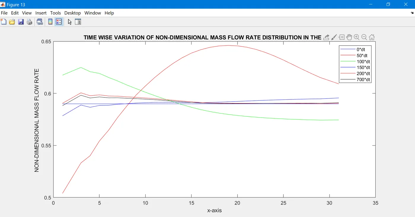
--> The initial mass flow is represented by (0*dt). The results after 100 time steps shows a somewhat "humped" distribution , after 200 time steps the mass flow distribution is becoming more constant value and is quite close to the value 0.579.
Comparing the steady-state result with the corresponding results obtained in non-conservation form it is evident that conservation form of the equation has more satisfactory mass flow results. The conservation form gives a distribution that is much closer to being a constant, in non-conservation form the mass flow results has a sizeable variation and some spurious oscillations at both inflow and outflow.
--> The conservation form does a better job of preserving the mass throughout the flow-field,mainly because the mass flow is one of the dependent variables in the equation or mass flow is the primary result of the equations.
COMPARISON OF CONSERVATION AND NON-CONSERVATION FOR OF GOVERNING EQUATIONS
1. The conservation form yields a better mass flow distribution.It does a better job at conserving mass.
2. The non-conservation form yields smaller residuals. The residual decay is often used as indexof "quality" of a numerical alogrithm.
3. There is no clear superiority of either forms in terms of the accuracy of the final solutions. The non-conservation form is more accurate for determining the primitive variables whereas the conservation form is more accurate to produce the results for the flux variables.
4. Solution of the conservation form requires more computational work (marginally) most of it is due to the decoding of the primitive variables into flux variables.
GRID-INDEPENDENCE TEST
--> When we solve the CFD problem we emoloy finite number of the grid points distributed over the domain of the flow field. We use N grid points and obtain a solution. Then we use 2N grid points, run the code and obtain new solutions.If both the solutions are practically the same and have very less marginal variations then our solution has achieved grid independence. However if the solution vary on a relatively large scale then our solution is a function of number of grid points, if we reach such a situation we should,if practicle,continue to increase grid points such that our solution is independent or no longer sensitive to the number of grid points.
clear all
close all
clc

% GRID INDEPENDENCE TEST
n=[31 61];

for i=1:2
x=linspace(0,3,n(i));
dx=x(2)-x(1);
gama=1.4;
nt=1000;% no. of time steps

%calculation of initial profile
rho= 1-0.3146*x;
T=1-0.2314*x;
v=(0.1 + 1.09*x).*T.^0.5;

% local sonic velocity
a1=(T).^0.5;

%area
a = 1 + 2.2*(x-1.5).^2;

% mass flow rate
m=(rho.*v).*a;

% times step
% (COURANT NUMBER)C=0.5
C=0.5;
%dt=0.0201;
dt1=C*(dx./(a1+v));
dt=min(dt1);

% outer time loop
for k=1:nt
    rho_old=rho;
    v_old=v;
    T_old=T;
    % predictor method
    for j=2:n(i)-1

        dvdxp=(v(j+1)-v(j))/dx;
        drhodxp=(rho(j+1)-rho(j))/dx;
        dTdxp=(T(j+1)-T(j))/dx;
        dlogadxp=(log(a(j+1)) - log(a(j)))/dx;

        % CONTINUITY EQUATION
        drhodt_p(j)= -rho(j)*dvdxp -rho(j)*v(j)*dlogadxp -v(j)*drhodxp;

        % MOMENTUM EQUATION
        dvdt_p(j)= -v(j)*dvdxp -(1/gama)*(dTdxp + ((T(j)*drhodxp)/(rho(j))));

        % ENERGY EQUATION
        dTdt_p(j)= -v(j)*dTdxp -(gama-1)*T(j)*(dvdxp + v(j)*dlogadxp);

        % solution update
        rho(j) = rho_old(j) + drhodt_p(j)*dt;
        v(j) = v_old(j) + dvdt_p(j)*dt;
        T(j) = T_old(j) + dTdt_p(j)*dt;
    end
    % corrector method
    for f=2:n(i)-1

        dvdx = (v(f)-v(f-1))/dx;
        drhodx = (rho(f)-rho(f-1))/dx;
        dTdx = (T(f)-T(f-1))/dx;
        dlogadx = (log(a(f))-log(a(f-1)))/dx;

        % CONTINUITY EQUATION
        drhodt_c(f)= -rho(f)*dvdx -rho(f)*v(f)*dlogadx -v(f)*drhodx;

        % MOMENTUM EQUATION
        dvdt_c(f)= -v(f)*dvdx -(1/gama)*(dTdx + ((T(f)*drhodx)/(rho(f))));

        % ENERGY EQUATION
        dTdt_c(f)= -v(f)*dTdx -(gama-1)*T(f)*(dvdx + v(f)*dlogadx);
    end
    % compute the average time derivative
    drhodt = 0.5*(drhodt_p + drhodt_c);
    dvdt = 0.5*(dvdt_p + dvdt_c);
    dTdt = 0.5*(dTdt_p + dTdt_c);

    %final solution update
    for j=2:n(i)-1
    rho(j) = rho_old(j) + drhodt(j)*dt;
    v(j) = v_old(j) + dvdt(j)*dt;
    T(j) = T_old(j) + dTdt(j)*dt;
    end

    %apply the boundary condition
    % inlet
    v(1) = 2*v(2) - v(3);
    %outlet
    v(n(i)) = 2*v(n(i)-1) - v(n(i)-2);
    rho(n(i)) = 2*rho(n(i)-1) - rho(n(i)-2);
    T(n(i)) = 2*T(n(i)-1) - T(n(i)-2);

    % mass flow rate
    m=(rho.*v).*a;
    % Mach number (M)
    M = v./(T.^0.5);
    % Non-dimensional Pressure
    P = rho.*T;

    % Update the value of time step
    a1=(T).^0.5;
    dt1=C*(dx./(a1+v));
    dt=min(dt1);
end
% Mach number (M)
M = v./(T.^0.5);
% Non-dimensional Pressure
P = rho.*T;

if i==2
    %nozzle_throat=31
    N_T=31;
    R1=rho(N_T);
    R2=T(N_T);
    R3=P(N_T);
    R4=M(N_T);
end
if i==1
    %nozzle_throat=16
    N_T=16;
    D1=rho(N_T);
    D2=T(N_T);
    D3=P(N_T);
    D4=M(N_T);
end
end
% Residue
rho_residue=R1-D1
T_residue=R2-D2
P_residue=R3-D3
M_residue=R4-D4
In the above alogrithm we see the difference between the values of primitive variables is marginally small and thus our solution is independent of number of grid points.