Week 1- Mixing Tee
Aim:-- To study the steady_state simulation of mixing of two air streams with different temperature and compare their mixing effectiveness. We check the mixing effectiveness for two different lengths(short and long pipe).
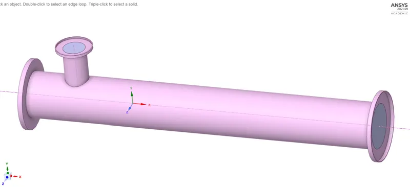
Mixing tees are very much used in the HVAC industries. As we can see the above model is set up for the mixing of single or multiple phases to allow heat transfer and also mass transfer. In the above model, we have two inlets with fluids entering at different temperatures (For our case fluid is "air"). Hot air flows in the main pipe and cold air flows through a tee. To measure the mixing effectiveness we calculate the standard deviation at the outlet. We also check for the mesh size and turbulence models used. Following are the two versions of the cases:--
- Case 1
- Short mixing tee with a hot inlet velocity of 3m/s.
- Momentum ratio of 2, 4.
- Case 2
- Long mixing tee with a hot inlet velocity of 3m/s.
- Momentum ratio of 2, 4.
Pre-Processing:--
1. Cad cleanup in Ansys SpaceClaim --> Our Cad model has many features that we do not need and therefore we only need the volume of flowing fluid. This is done by using the volume extract option on the prepare tab.
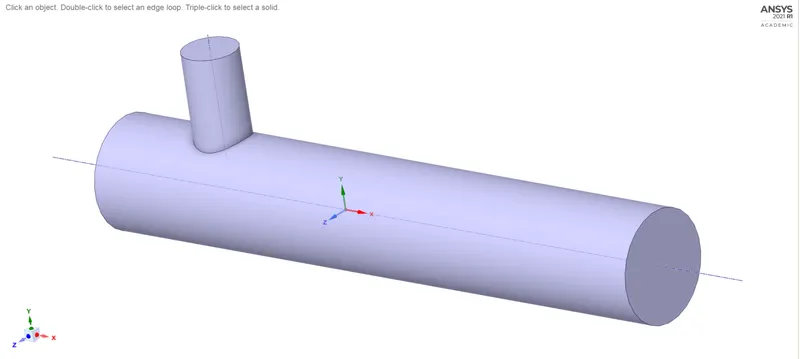
2. Generating Mesh (Ansys Meshing module) and case setup in Ansys fluent --> In Ansys meshing we generate the mesh and we also give names to the boundaries. In Ansys fluent we setup the boundary condition, steady-state solver, initialization and solving the equations. We also generate the report and plot files about the field variables for analysis.
Defining some variables:--
1. velocity of hot air --> V_h
2. velocity of cold air --> V_c
3. Temperature of hot air --> T_h
4. Temperature of cold air --> T_c
CASE 1]
Momentum ratio of 2.
T_h = 36 degree celsius (inlet_x)
T_c = 19 degree celsius (inlet_y)
V_h = 3 m/s
V_c = 6 m/s (Momentum ratio=2)
Turbulence model = k-ε Relizable model.
Following are the mesh/setup/results plots -->
Mesh size = 0.002 m.
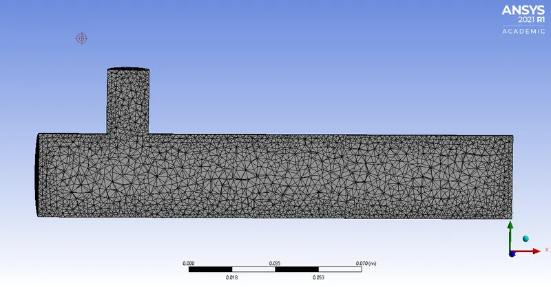
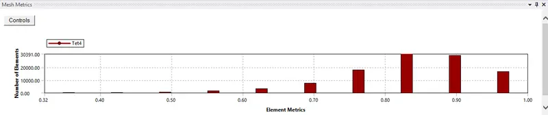
Mesh metric plot
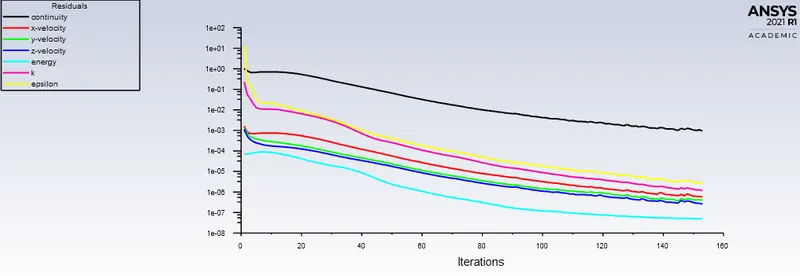
Residual plot.
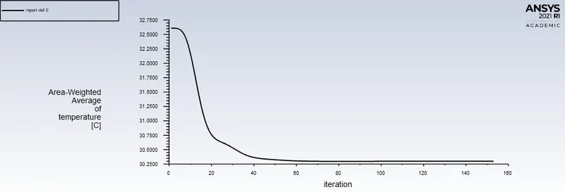
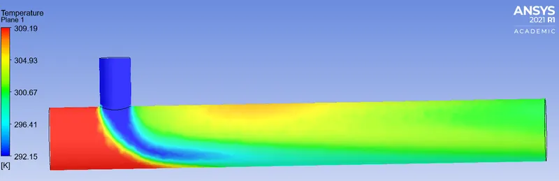
Average Temperature.
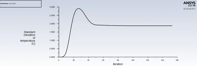
The standard deviation of temperature.
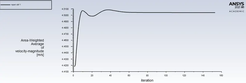
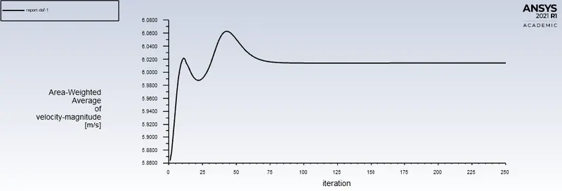
Average velocity.
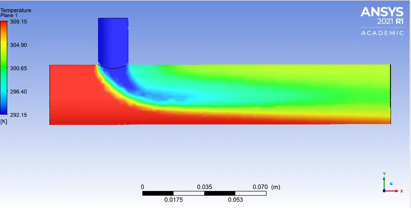
Temperature variation along the axial plane.
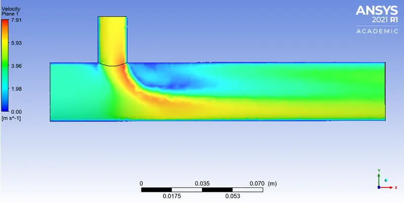
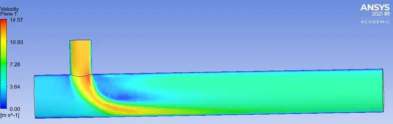
Velocity Variation along the axial plane.
Momentum ratio 2, Turbulence Model (k-ω SST)
T_h = 36 degree celsius (inlet_x)
T_c = 19 degree celsius (inlet_y)
V_h = 3 m/s
V_c = 6 m/s (Momentum ratio=2)
Turbulence model = k-ω SST model.
Following are the mesh/setup/results plots -->
Mesh size = 0.002 m.(Mesh plots are the same as before)
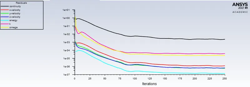
Residual plot
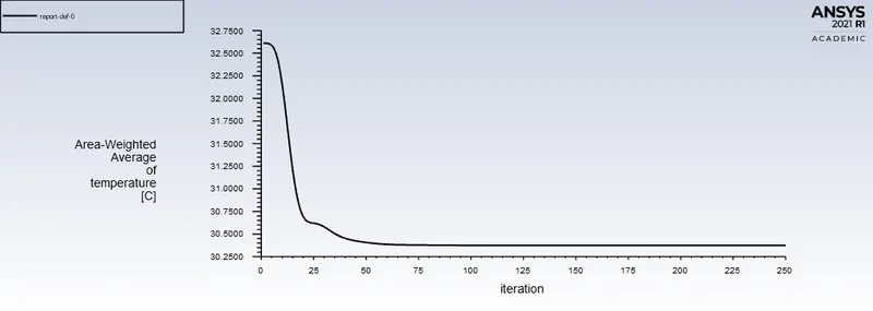
Avg. Temperature
Standard deviation
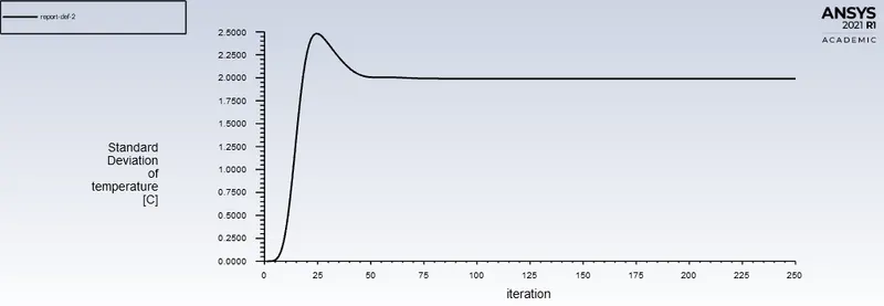
Avg. velocity
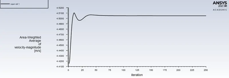
Momentum ratio of 4.
T_h = 36 degree celsius (inlet_x)
T_c = 19 degree celsius (inlet_y)
V_h = 3 m/s
V_c = 12 m/s (Momentum ratio=4)
Turbulence model = k-ε Relizable model.
Following are the mesh/setup/results plots -->
Mesh size = 0.002 m.(Mesh plots are the same as before)
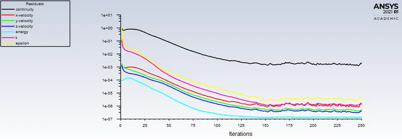
Residual plot
Avg. Temperature
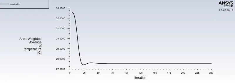
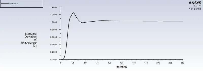
Standard deviation
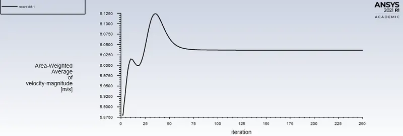
Avg. velocity
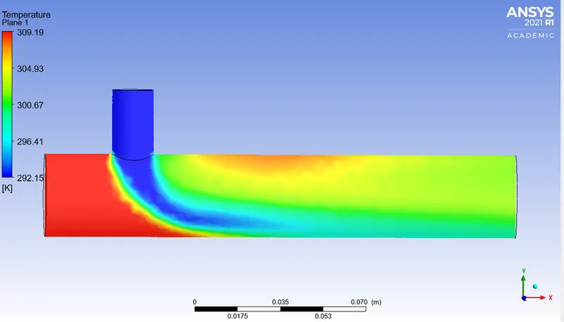
Temperature plot along the axial plane
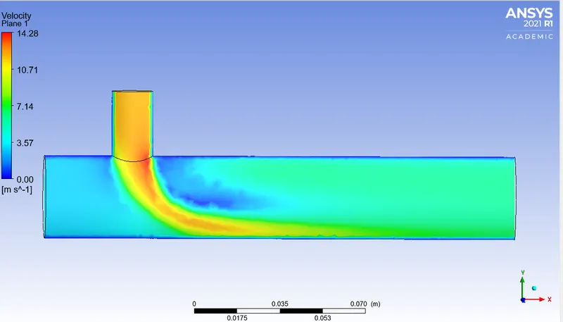
Velocity plot along the axial plane
CASE 2]
Momentum ratio of 2.
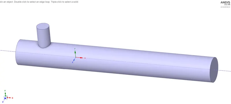
Cad for 2nd case -->
T_h = 36 degree celsius (inlet_x)
T_c = 19 degree celsius (inlet_y)
V_h = 3 m/s
V_c = 6 m/s (Momentum ratio=2)
Turbulence model = k-ε Relizable model.
Following are the mesh/setup/results plots -->
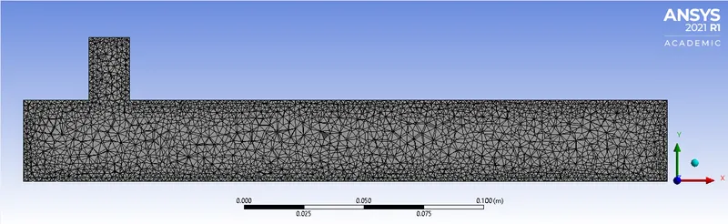
Mesh size = 0.002 m.
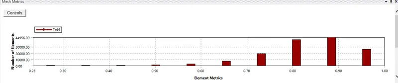
Mesh metric plot
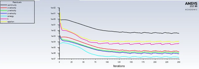
Scaled residual plot
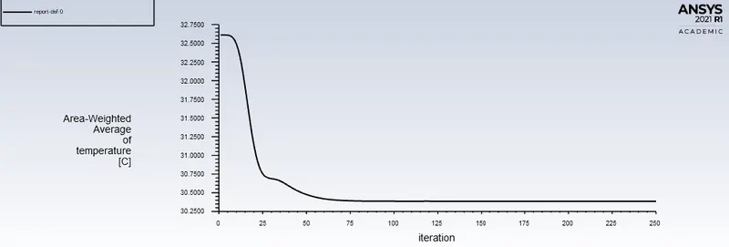
Avg. Temperature
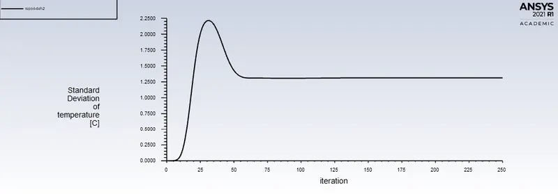
The standard deviation of Temperature
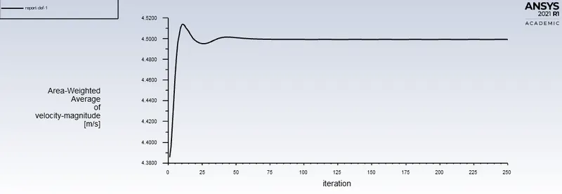
Avg. Velocity
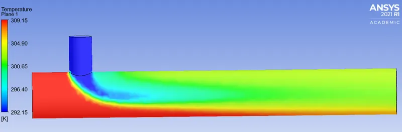
Temperature plot along the axial plane
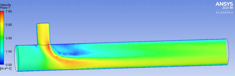
Velocity plot along the axial plane
Momentum ratio of 4.
T_h = 36 degree celsius (inlet_x)
T_c = 19 degree celsius (inlet_y)
V_h = 3 m/s
V_c = 12 m/s (Momentum ratio=4)
Turbulence model = k-ε Relizable model.
Following are the mesh/setup/results plots -->
Mesh size = 0.002 m.
(Mesh plots are similar as shown previously)
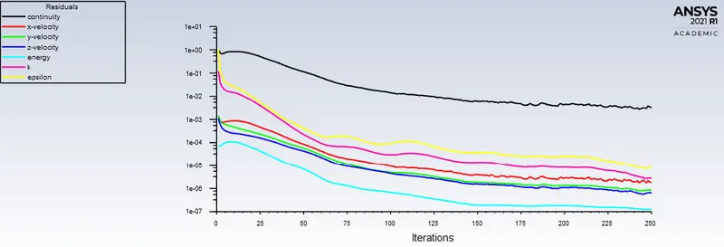
Scaled residuals plot
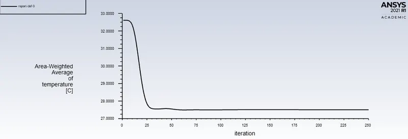
Avg. Temperature
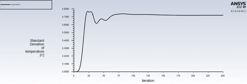
Standard deviation of Temperature
Avg. Velocity
Temperature plot along the axial plane
Velocity plot along the axial plane
| Case I - Short Tee | Momentum Ratio | Turbulence Model | Cell count. |
Avg. Temperature (degree Celsius) |
Standard deviation |
Iteration Number (Convergence) |
| 2 | k-ε Relizable model | 106152 | 30.298 | 1.87 | 50 | |
| 2 | k-ω SST model | 106152 | 30.374 | 1.98 | 50 | |
| 4 | k-ε Relizable model | 106152 | 27.562 | 1.02 | 70 | |
| Case II - Long Tee | ||||||
| 2 | k-ε Relizable model | 141712 | 30.3 | 1.25 | 70 | |
| 4 | k-ε Relizable model | 141712 | 27.4 | 0.7 | 75 |
Conclusion -->
1. The Average temperature at the outlet drops down due to the increase in the velocity of cold air. We also have a low value for standard deviation, which means mixing is more efficient (because of turbulent mixing). Therefore, high momentum ratio will ensure more mixing and temperature reduction.
2. If we use longer then the temperature contour at the outlet will be more uniform. As we can see in short pipes hot air can slip through at the bottom (as a result of improper mixing), so longer pipes will ensure uniform temperature distribution at the outlet.
3. We use two turbulence models ( k-ε Relizable model and k-ω SST model ). The k-ε model is good to predict far away from the wall. This is in general for internal fluid flows where near-wall considerations are not important. k-ω SST model predicts good near the wall, it is especially used for external fluid flows (aerodynamic) so we continue to use the k-ε Relizable model for modelling turbulence.
The following video demonstrates all cases discussed above.