Week 5 - Mid term project - Solving the steady and unsteady 2D heat conduction problem
clear all
close all
clc

% code for solving II order PDE (heat conduction) by using point itERATIVE
% TECHNIQUE
% BC's
% top face = 600 K
% bottom face = 900 K
% left face = 400 K
% right face = 800 k
% Equation --> [d^2(T)/dx^2] + [d^2(T)/dy^2] = 0    2-D heat conduction
% equation


w = 1.2; % sucessive over-relaxation factor
nx=10;
ny=10;
x=linspace(0,1,nx);
y=linspace(0,1,ny);
% defining "K" , "dx" , "dy".
dx = x(2)-x(1);
dy = y(2)-y(1);
K = 2*((dx^2 + dy^2)/(dx*dy)^2);
% defining the temperature field in 2D
T = ones(ny,nx);
% implementing the boundary conditions
T(1,2:nx-1) = 600;
T(ny,2:nx-1) = 900;
T(2:ny-1,1) = 400;
T(2:ny-1,nx) = 800;
T(1,1) = 500;
T(1,nx) = 700;
T(ny,1) = 650;
T(ny,nx) = 850;
% creating a copy of dependent variable
Told = T;
T_initial = T;


iterative_solvers=2;


%jacobi iteration
if iterative_solvers == 1
    error = 1e1;
    tol=1e-4;
    jacobi_iter = 1;
   while(error > tol)
   for i=2:nx-1
       for j=2:ny-1
       T(i,j) = (Told(i+1,j) + Told(i-1,j))/(K*(dx)^2) + (Told(i,j+1) + Told(i,j-1))/(K*(dy)^2);
       end
   end
   error = max(max(abs(Told-T)));
   Told=T; % update the velocity
   jacobi_iter = jacobi_iter + 1;
   surf(x,y,T)
   colormap(jet(50))
   colorbar
   grid on
   pause(0.03)
   xlabel('x-axis')
   ylabel('y-axis')
   zlabel('JACOBI   METHOD   TEMPERATURE    T(x,y)')
   title_text = sprintf('iteration number = %d',jacobi_iter);
   title(title_text)
   end
end

%GS iteration
if iterative_solvers == 2
    error = 1e1;
    tol=1e-4;
    gs_iter = 1;
   while(error > tol)
   for i=2:nx-1
       for j=2:ny-1
       T(i,j) = (Told(i+1,j)+T(i-1,j))/(K*(dx)^2) + (Told(i,j+1)+T(i,j-1))/(K*(dy)^2);
       end
   end
   error = max(max(abs(Told-T)));
   Told=T; % update the velocity
   gs_iter = gs_iter + 1;
   surf(x,y,T)
   colormap(jet(50))
   colorbar
   grid on
   pause(0.03)
   xlabel('x-axis')
   ylabel('y-axis')
   zlabel('GAUSS SEIDAL   METHOD   TEMPERATURE    T(x,y)')
   title_text = sprintf('iteration number = %d',gs_iter);
   title(title_text)
   end
end


% SOR successive overrelaxation method
if iterative_solvers == 3
    error = 1e1;
    tol=1e-4;
    SOR_iter = 1;
   while(error > tol)
   for i=2:nx-1
       for j=2:ny-1
       T(i,j) = (1-w)*Told(i,j) + w*((Told(i+1,j) + T(i-1,j))/(K*(dx)^2) + (Told(i,j+1) + T(i,j-1))/(K*(dy)^2));
       end
   end
   error = max(max(abs(Told-T)));
   Told=T; % update the velocity
   SOR_iter = SOR_iter + 1;
   surf(x,y,T)
   colormap(jet(50))
   colorbar
   grid on
   pause(0.03)
   xlabel('x-axis')
   ylabel('y-axis')
   zlabel('SOR   METHOD   TEMPERATURE    T(x,y)')
   title_text = sprintf('iteration number = %d',SOR_iter);
   title(title_text)
   end
end
clear all
close all
clc

% Explicit methods
% code for solving II order PDE (Unsteady or transient heat conduction)
% Equation --> a[d^2(T)/dx^2] + a[d^2(T)/dy^2] = [dT/dt]
% a = thermal diffusivity = 1.4

nx=10;
ny=10;
x=linspace(0,1,nx);
y=linspace(0,1,ny);

% defining "K1" , "K2" , "a" , "dx" , "dy"
a = 1.4;
dx = x(2)-x(1);
dy = y(2)-y(1);
dt = 0.002;
k1 = (a*dt)/(dx)^2;
K2 = (a*dt)/(dy)^2;

% defining the temperature field in 2D
T = ones(ny,nx);

% implementing the boundary conditions
T(1,2:nx-1) = 600;
T(ny,2:nx-1) = 900;
T(2:ny-1,1) = 400;
T(2:ny-1,nx) = 800;
T(1,1) = 500;
T(1,nx) = 700;
T(ny,1) = 650;
T(ny,nx) = 850;

% creating a copy of dependent variable
Told = T;

% Time loop
nt = 1400;
for k=1:nt
    %space loop
    for i=2:nx-1
        for j=2:ny-1
        T(i,j) = Told(i,j) + k1*(Told(i+1,j)-(2*Told(i,j))+Told(i-1,j)) + K2*(Told(i,j+1)-(2*Told(i,j))+Told(i,j-1));
        end
    end
    Told=T;% updating the temperature profile
    contourf(x,y,T,'LineStyle','none')
    set(gca,'YDIR','reverse')
    colormap(jet(50))
    colorbar
    pause(0.00000000003)
    xlabel('x-axis')
    ylabel('y-axis')
end
clear all
close all
clc
% implicit methods
% code for solving II order PDE (Unsteady or transient heat conduction)
% Equation --> a[d^2(T)/dx^2] + a[d^2(T)/dy^2] = [dT/dt]
% a = thermal diffusivity = 1.4
w=1.1;
a = 1.4;
nx=10;
ny=10;
x=linspace(0,1,nx);
y=linspace(0,1,ny);
% defining "K1" , "K2" , "a" , "dx" , "dy"
dx = x(2)-x(1);
dy = y(2)-y(1);
dt = 0.0015;
k1 = (a*dt)/(dx)^2;
K2 = (a*dt)/(dy)^2;
term1 = (1 + (2*k1) + (2*K2))^(-1);
term2 = k1*term1;
term3 = K2*term1;
% defining the temperature field in 2D
T = ones(ny,nx);
% implementing the boundary conditions
T(1,2:nx-1) = 600;
T(ny,2:nx-1) = 900;
T(2:ny-1,1) = 400;
T(2:ny-1,nx) = 800;
T(1,1) = 500;
T(1,nx) = 700;
T(ny,1) = 650;
T(ny,nx) = 850;
% creating a copy of dependent variable for the current time step iteration
Told = T;
% creating a copy of dependent variable for previous time step
T_prev=T;
Iterative_solvers = 3;
if Iterative_solvers == 1 %jacobi iteration
% Time loop
nt = 1400;
for k=1:nt
error = 1e1;
tol = 1e-4;
% convergence loop
while(error > tol)
%space loop
for i=2:nx-1
for j=2:ny-1
T(i,j) = (term1)*T_prev(i,j) + (term2)*(Told(i+1,j) + Told(i-1,j)) + (term3)*(Told(i,j+1) + Told(i,j-1));
end
end
error = max(max(abs(Told-T)));
Told=T;% updating the temperature profile for iteration
end
T_prev = T;
end
contourf(x,y,T,'LineStyle','none')
set(gca,'YDIR','reverse')
colormap(jet(50))
colorbar
end
if Iterative_solvers == 2 % GS iteration
% Time loop
nt = 1400;
for k=1:nt
error = 1e1;
tol = 1e-4;
% convergence loop
while(error > tol)
%space loop
for i=2:nx-1
for j=2:ny-1
T(i,j) = (term1)*T_prev(i,j) + (term2)*(Told(i+1,j) + T(i-1,j)) + (term3)*(Told(i,j+1) + T(i,j-1));
end
end
error = max(max(abs(Told-T)));
Told=T;% updating the temperature profile for iteration
end
T_prev = T;
end
contourf(x,y,T,'LineStyle','none')
set(gca,'YDIR','reverse')
colormap(jet(50))
colorbar
end
if Iterative_solvers == 3 % SOR iteration
% Time loop
nt = 1400;
for k=1:nt
error = 1e1;
tol = 1e-4;
% convergence loop
while(error > tol)
%space loop
for i=2:nx-1
for j=2:ny-1
T(i,j) = (1-w)*Told(i,j) + w*((term1)*T_prev(i,j) + (term2)*(Told(i+1,j) + T(i-1,j)) + (term3)*(Told(i,j+1) + T(i,j-1)));
end
end
error = max(max(abs(Told-T)));
Told=T;% updating the temperature profile for iteration
end
T_prev = T;
end
contourf(x,y,T,'LineStyle','none')
set(gca,'YDIR','reverse')
colormap(jet(50))
colorbar
endSTEADY STATE AND TRANSIENT STATE ANALYSIS
[1]. STEADY STATE -- STEADY STATE 2-D HEAT CONDUCTION EQUATION
∂^2[T]/∂(x)^2 + ∂^2[T]/∂(y)^2 = 0
--> We are given an steady state heat conduction equation in 2 dimensions. This is a partial differential equation. It is an elliptic Partial differential equation, In elliptic PDE information travels at infinite speed inside the domain in all direction inside the domain. We discretize the above PDE by using taylors II order accurate central difference method in both terms (x and y).
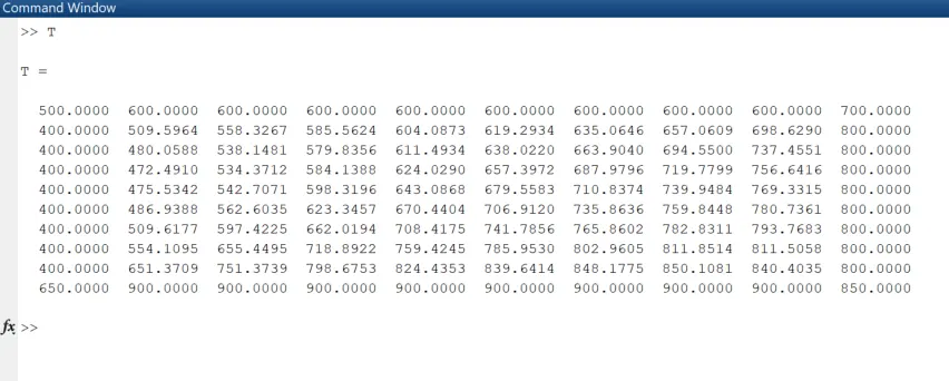
--> Now we implement the boundary condition and solve the difference equations by using point iterative technique. Following are the point iteration technique, these techniques are like shooting method, from an initial guess we converge our results to actual solution.
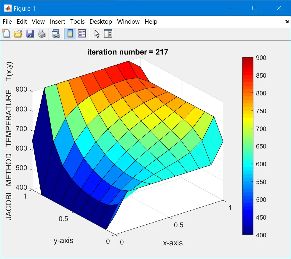
1 Jacobi technique -- In this iterative technique we compute new guess values for dependent variable by strictly using the old iterative value.
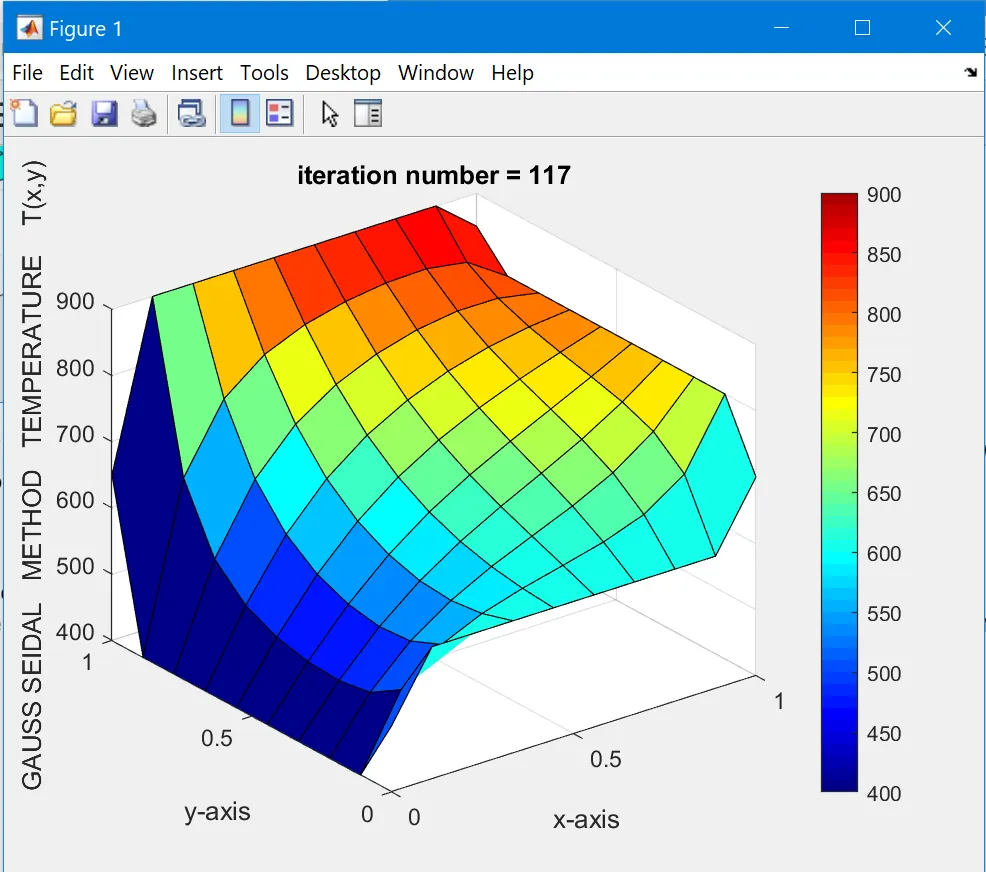
2 Gauss seidal method [GS] -- In this iterative technique as we compute new guess values for dependent variable we update the values for the dependent variable by this method of updating the values we converge to the result faster.
3 sucessive over-relaxation technique [SOR] -- In SOR we multiply the rate of convergence by a number (grater than 1) which is called relaxation factor that over-shoots the convergence rate in order to converge faster then the previous methods (gauss seidal and jacobi method).
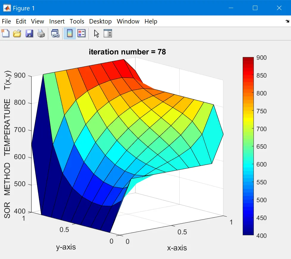
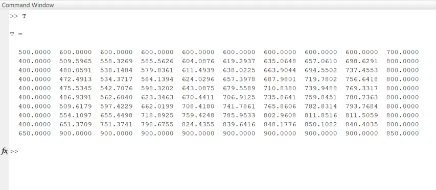
solution matrix for temperature-->
SOR METHOD
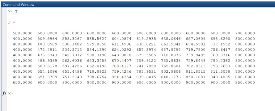
JACOBI METHOD
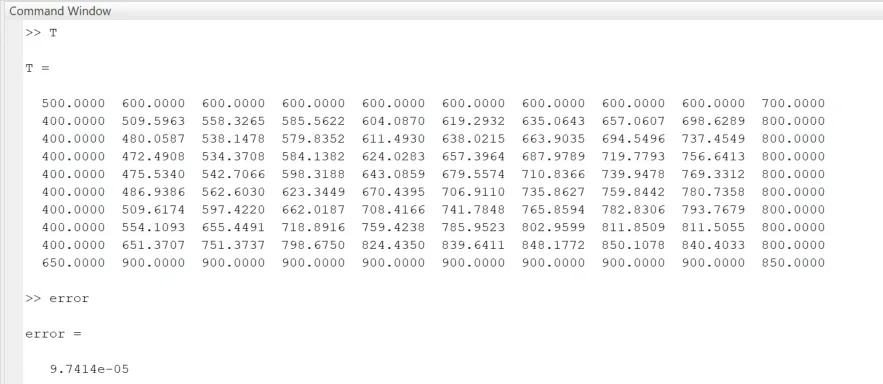
GAUSS-SEIDAL METHOD
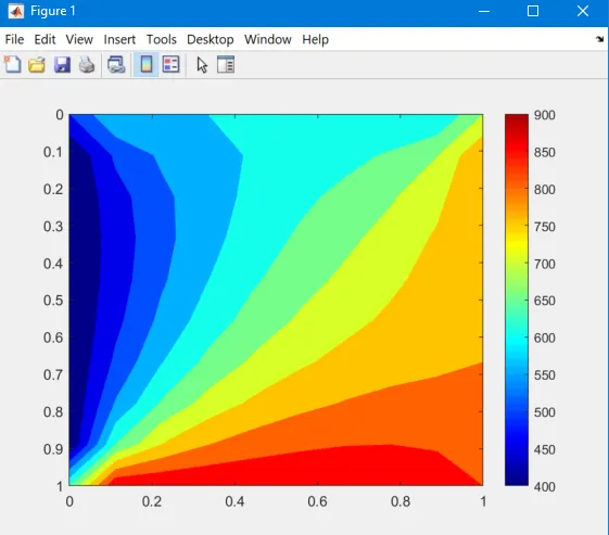
[2]. Transient state 2-D heat conduction equation
α [ ∂^2[T]/∂(x)^2 + ∂^2[T]/∂(y)^2 ] = ∂T/∂t
UNSTEADY STATE HEAT CONDUCTION EQUATION where α = thermal diffusivity = 1.4