Week 11 - Simulation of Flow through a pipe in OpenFoam

SIMULATION OF LAMINAR PIPE-FLOW IN OPENFOAM

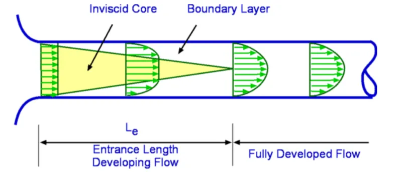
--> In this project we are going to analyse fluid flowing in the pipe and compare computational result (obtained in openFoam) with analytical hagen-poiseuille equation for laminar pipe flow. In the process we are going to capture the laminar Boundary layer development at the Entrance region (where the fluid flow is developing) and also the hydrodynamically fully-developd region (where the momentm and velocity profile does not change along the flow direction).The length of the Entrance region is called Entrance length (Le).

Analysing the Hagen-Poiseuille (HP) equation for Pipe Flow:--

--> When a viscous fluid flows on a solid surface the fluid velocity is zero at the solid surface as the molecules get stuck at the surface (no-slip boundary condition).This gives rise to Momentum disturbance which causes the adjacent layer to slow down and a velocity gradient () is formed along radial direction. The property by virtue of which this effect propages in the flow is called Viscosity.

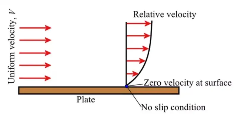
All real fluid are viscous in nature. The region upto which the effect of wall is felt is called the boundary layer region or viscous region. The region outside is inviscid flow. As we move away from solid surface the viscous forces are very low and effect of wall is very less. To maintain the continuity of Mass flow the flow in inviscid core must be accelerating and axial velocity must exceed free stream velocity to a maximum value.

--> After the flow becomes FDF (Fully-developed flow) the velocity profile does not change and becomes constant(as shown in the figure).

Geometry and Assumptions:--

Diameter of the pipe -- D = 0.1 m = 10 cm

Reynold's Number -- Re = [D*v(avg)]/nu It must be less than 2100 for laminar flow (otherwise the flow will take transition to turbulance)

Working fluid --- Water at temperature 298 (degree kelvin).

Dynamic Viscosity --- mu = 8.4e-4 Pa.s

Density of Water --- rho = 997 Kg/m3

Kinematic Viscosity --- nu = 8.42527e-7 m2/s

Initial uniform velocity --- v = [nu*Re]/D ---> v = 0.0169 m/s

--- V(max) = 2*v = 0.0337 m/s

Entrance Length --- Le = 0.05*Re*D = 0.05*2000*0.1 = 10 m

Pressure drop △p --- △p= (32*mu*L*v)/(D)^2 = 6.7941 Pa

Kinematic Pressure drop --- △p(kinematic) = △p/rho = 0.0068 m

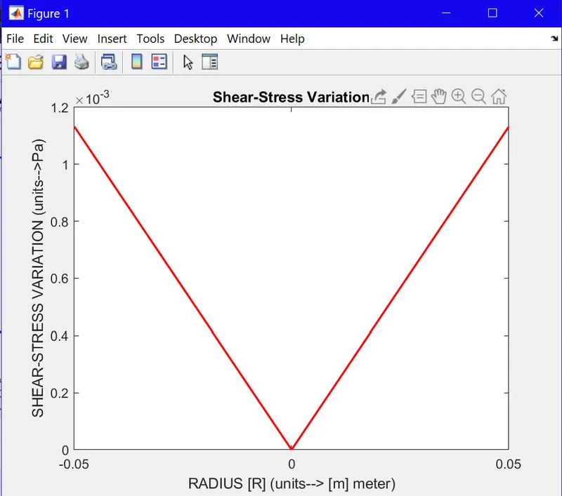
Shear stress --- τ = (4*mu*v)/r = 0.0011 Pa

The following MATLAB code will solve the Pipe Flow problem using Hagen-Poiseuille Equations and will give analytical values for flow variables, with all the variation plotted in the Graphs.

clear all 
close all
clc
% input geometry of Pipe
d=0.1; % unit--> [m] meters
R=d/2;
L=150; % unit--> [m] meters
% Co-ordinates of Wedge Points
x_pt=R*cosd(1);
y_pt=R*sind(1);

% Fluid properties Fixed values 
nu=8.42527e-7; % Kinematic Viscosity --> [m^2/s]
rho=997; % Density --> [Kg/m^3]
Re=2000; % For Laminar Flow [Re<=2100]
mu=nu*rho; % Dynamic Viscosity --> [Kg/m*s]
% Calculation of the flow variables
Le=(0.05*Re*d); % Entrance Length for laminar Flow
v=(Re*nu)/d; % Avg. velocity at entrance
vmax=2*v; % Maximum velocity
deltaP=(32*v*L*mu)/(d^2); % Pressure Drop along the length (Pa pascals)
K_dP = deltaP/rho; % Kinematic Pressure (unit--> meters (m)).
tau_wall=(4*mu*v)/R; % wall shear-stress

% Analytical Results
% plotting shear-stress as a function of radius
o=6;
Tau_1=ones(1,o);
Tau_2=ones(1,o);
r_1=linspace(0,0.05,o);
r_2=linspace(0,-0.05,o);
for k=1:o
for i=1:o
    Tau_1(i)=(4*mu*v*r_1(i))/(R^2);
    Tau_2(k)=-(4*mu*v*r_2(k))/(R^2);
end
end
figure(1)
plot(r_1,Tau_1,'r','linewidth',1.5)
hold on 
plot(r_2,Tau_2,'r','linewidth',1.5)
xlabel('RADIUS [R] (units--> [m] meter)')
ylabel('SHEAR-STRESS VARIATION (units-->Pa)')
title('Shear-Stress Variation')

% Fully-Developed Velocity profile Variation 
% Given by Hagen-Poiseuille Equation for Laminar Pipe Flow
c=20;
r1=linspace(0,0.05,c);
r2=linspace(0,-0.05,c);
V_r_1=ones(1,c);
V_r_2=ones(1,c);
for i=1:c
    for k=1:c
        V_r_1(i) = 2*v*(1 - (r1(i)/R)^2);
        V_r_2(k) = 2*v*(1 - (r2(k)/R)^2);
    end
end
figure(2)
plot(V_r_1,r1,'b','linewidth',1.5)
hold on 
plot(V_r_2,r2,'b','linewidth',1.5)
xlabel('RADIUS [R] (units--> [m] meter)')
ylabel('VELOCITY VARIATION (units--> m/s)')
legend('Vmax = 0.033701 m/s')
title('Fully-Developed Pipe Flow By H-P equation')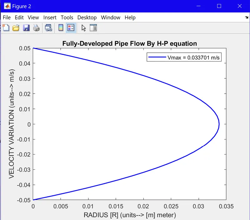

close all 
clear all
clc
% Geometry of the pipe(Length and Diameter)
L=150;
d=0.1;
% Input Wedge Angle
thita=input("Enter the wedge angle--> ");
% Co-ordinates of the Wedge Section
x_pt= (d/2)*cosd(thita/2);
y_pt= (d/2)*sind(thita/2);
% Input scaling factors
sf_x=input("Enter the grading factor for x-axis--> ");
sf_y=input("Enter the grading factor for y-axis--> ");
sf_z=input("Enter the grading factor for z-axis--> ");
% Writing Strings for the BlockMeshDict File
foamFile = sprintf("FoamFile\n{\n    version    %s; \n    format     ascil; \n    class      dictionary; \n    object     blockMeshDict; \n}",'2.0');
scale = sprintf(" \nconvertToMeters  %d;",1);
vertices = sprintf("\nvertices\n(\n(0 0 0)\n(%d %d 0)\n(%d -%d 0)\n(0 0 %d)\n(%d %d %d)\n(%d -%d %d)\n);",x_pt,y_pt,x_pt,y_pt,L,x_pt,y_pt,L,x_pt,y_pt,L);
block = sprintf("\nblocks\n(\n    hex(0 2 1 0 3 5 4 3) (50 1 200) simpleGrading (%d %d %d)\n);",sf_x,sf_y,sf_z);
edge = sprintf("\nedges\n(\n    arc 1 2 (%d 0 0)\n    arc 4 5 (%d 0 %d)\n);",d/2,d/2,L);
boundary = sprintf("\nboundary\n(\n    inlet\n    {\n        type patch;\n        faces\n        (\n        (0 1 2 0)\n        );\n    }\n    outlet\n    {\n        type patch;\n        faces\n        (\n        (3 5 4 3)\n        );\n    }\n    tankWall\n    {\n        type wall;\n        faces\n        (\n        (1 4 5 2)\n        );\n    }\n    front\n    {\n        type wedge;\n        faces\n        (\n        (0 3 4 1)\n        );\n    }\n    back\n    {\n        type wedge;\n        faces\n        (\n        (0 2 5 3)\n        );\n    }\n    axis\n    {\n        type symmetry;\n        faces\n        (\n        (0 3 3 0)\n        );\n    }\n);");
merge = sprintf("\nmergePatchPairs\n(\n);");
% Combining all the above strings in single array.
blockMeshDictString = strcat(foamFile , scale , vertices , block , edge , boundary , merge);
% Generating blockMeshDict File.
file = fopen('blockMeshDict', 'w');
fprintf(file,'%s',blockMeshDictString);
fclose(file);

--> The following .txt are the various dictionary files used to run the case setup in openFoam. BlockMeshDict generates the geometry and meshes it. We create a wedge of angle 2 degree and use wedge boundary conditionon the faces and simulate the flow for that wedge geometry.

/*--------------------------------*- C++ -*----------------------------------*\
  =========                 |
  \\      /  F ield         | OpenFOAM: The Open Source CFD Toolbox
   \\    /   O peration     | Website:  https://openfoam.org
    \\  /    A nd           | Version:  8
     \\/     M anipulation  |
\*---------------------------------------------------------------------------*/
FoamFile
{
    version     2.0;
    format      ascii;
    class       dictionary;
    object      blockMeshDict;
}
// * * * * * * * * * * * * * * * * * * * * * * * * * * * * * * * * * * * * * //


convertToMeters 1;

vertices
(
    (0 0 0)
    (0.04999238 8.7267e-4 0)
    (0.04999238 -8.7267e-4 0)
    (0 0 150)
    (0.04999238 8.7267e-4 150)
    (0.04999238 -8.7267e-4 150)
);

blocks
(
    hex (0 2 1 0 3 5 4 3) (50 1 200) simpleGrading (2 1 1)
);

edges
(
    arc 1 2 (0.05 0 0)
    arc 4 5 (0.05 0 150)
);

boundary
(
    inlet
    {
        type patch;
        faces
        (
            (0 1 2 0)
        );
    }
    outlet
    {
        type patch;
        faces
        (
            (3 5 4 3)
        );
    }
    tankWall
    {
        type wall;
        faces
        (
            (1 4 5 2)
        );
    }
    front
    {
        type wedge;
        faces
        (
            (0 3 4 1)
        );
    }
    back
    {
        type wedge;
        faces
        (
            (0 2 5 3)
        );
    }    
    axis
    {
        type symmetry;
        faces
        (
            (0 3 3 0)
        );
    }
);

mergePatchPairs
(
);

// ************************************************************************* //

/*--------------------------------*- C++ -*----------------------------------*\
  =========                 |
  \\      /  F ield         | OpenFOAM: The Open Source CFD Toolbox
   \\    /   O peration     | Website:  https://openfoam.org
    \\  /    A nd           | Version:  8
     \\/     M anipulation  |
\*---------------------------------------------------------------------------*/
FoamFile
{
    version     2.0;
    format      ascii;
    class       dictionary;
    location    "system";
    object      controlDict;
}
// * * * * * * * * * * * * * * * * * * * * * * * * * * * * * * * * * * * * * //

application     icoFoam;

startFrom       startTime;

startTime       0;

stopAt          endTime;

endTime         1000;

deltaT          1;

writeControl    timeStep;

writeInterval   20;

purgeWrite      0;

writeFormat     ascii;

writePrecision  6;

writeCompression off;

timeFormat      general;

timePrecision   6;

runTimeModifiable true;


// ************************************************************************* //

/*--------------------------------*- C++ -*----------------------------------*\
  =========                 |
  \\      /  F ield         | OpenFOAM: The Open Source CFD Toolbox
   \\    /   O peration     | Website:  https://openfoam.org
    \\  /    A nd           | Version:  8
     \\/     M anipulation  |
\*---------------------------------------------------------------------------*/
FoamFile
{
    version     2.0;
    format      ascii;
    class       dictionary;
    location    "constant";
    object      transportProperties;
}
// * * * * * * * * * * * * * * * * * * * * * * * * * * * * * * * * * * * * * //

nu              [0 2 -1 0 0 0 0] 8.42527e-7;


// ************************************************************************* //

/*--------------------------------*- C++ -*----------------------------------*\
  =========                 |
  \\      /  F ield         | OpenFOAM: The Open Source CFD Toolbox
   \\    /   O peration     | Website:  https://openfoam.org
    \\  /    A nd           | Version:  8
     \\/     M anipulation  |
\*---------------------------------------------------------------------------*/
FoamFile
{
    version     2.0;
    format      ascii;
    class       volVectorField;
    object      U;
}
// * * * * * * * * * * * * * * * * * * * * * * * * * * * * * * * * * * * * * //

dimensions      [0 1 -1 0 0 0 0];

internalField   uniform (0 0 0);

boundaryField
{
    tankWall
    {
        type            noSlip;
    }

    inlet
    {
        type            fixedValue;
        value           uniform (0 0 0.0169);
    }

    outlet
    {
        type            zeroGradient;
    }

    front
    {
        type            wedge;
    }

    back
    {
        type            wedge;
    }

    axis
    {
        type            symmetry;
    }
}

// ************************************************************************* //

/*--------------------------------*- C++ -*----------------------------------*\
  =========                 |
  \\      /  F ield         | OpenFOAM: The Open Source CFD Toolbox
   \\    /   O peration     | Website:  https://openfoam.org
    \\  /    A nd           | Version:  8
     \\/     M anipulation  |
\*---------------------------------------------------------------------------*/
FoamFile
{
    version     2.0;
    format      ascii;
    class       volScalarField;
    object      p;
}
// * * * * * * * * * * * * * * * * * * * * * * * * * * * * * * * * * * * * * //

dimensions      [0 2 -2 0 0 0 0];

internalField   uniform 0;

boundaryField
{
    tankWall
    {
        type            zeroGradient;
    }

    inlet
    {
        type            zeroGradient;
    }

    outlet
    {
        type            fixedValue;
        value           uniform 0;
    }

    front
    {
        type            wedge;
    }

    back
    {
        type            wedge;
    }

    axis
    {
        type            symmetry;
    }
}

// ************************************************************************* //

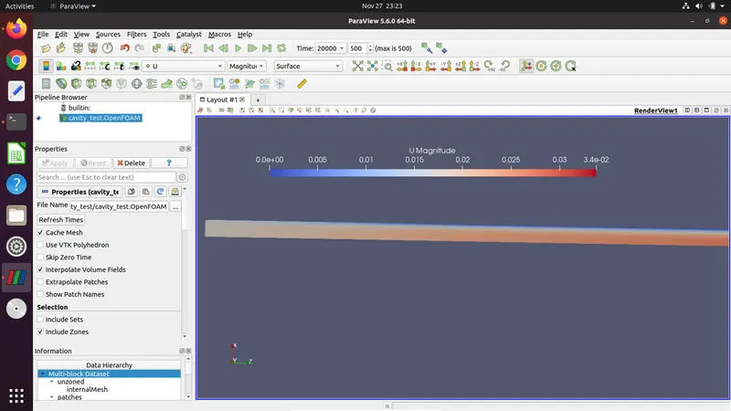
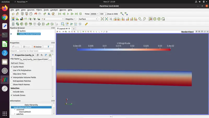
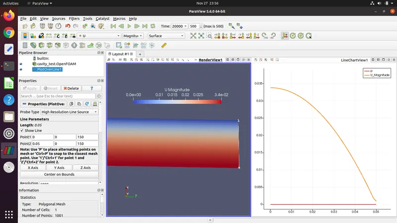
--> After running the icoFoam solver in openFoam we get the following results.

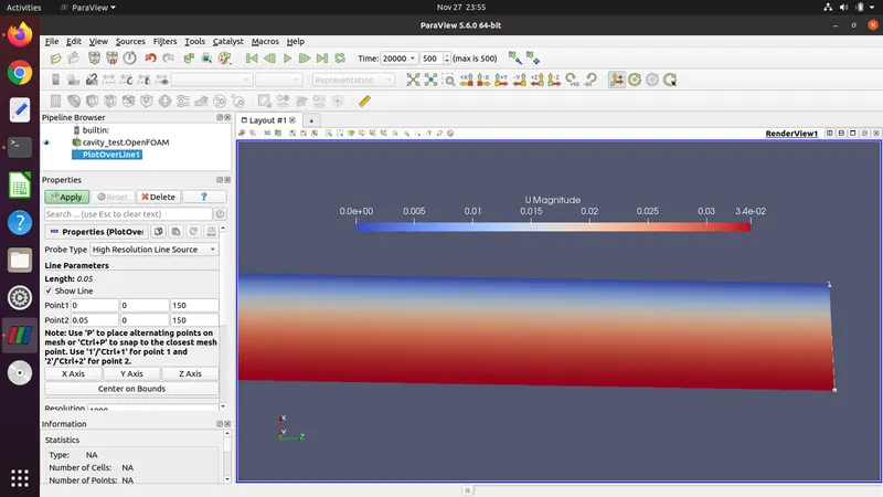
Following is the MATLAB code for reading and plotting the .csv files that were generated from paraView in openFoam.

clear all
close all
clc
% Plotting velocity profile for radius 20 m  
V_x_1=xlsread('v_Fuly_Developed_profile.csv','v_Fuly_Developed_profile','A1:A1002'); % x-component of velocity
V_y_1=xlsread('v_Fuly_Developed_profile.csv','v_Fuly_Developed_profile','B1:B1002'); % y-component of velocity
V_z_1=xlsread('v_Fuly_Developed_profile.csv','v_Fuly_Developed_profile','C1:C1002'); % z-component of velocity
r_pt=xlsread('v_Fuly_Developed_profile.csv','v_Fuly_Developed_profile','G2:G1001'); % points along the radius
r_pt_negative= (-r_pt);
U_mag_1=(V_x_1.^2 + V_y_1.^2 + V_z_1.^2).^(1/2);
figure(1)
plot(U_mag_1,r_pt,'r','linewidth',1.5)
hold on
plot(U_mag_1,r_pt_negative,'r','linewidth',1.5)
grid on
ylabel('Pipe Radius (m)')
xlabel('Velocity (m/s)')
legend('Vmax = 0.033755')
title('FULLY DEVELOPED VELOCITY PROFILE at 20m.')

% Plotting velocity profile for radius 15 m  
V_x_2=xlsread('v_profile_15.csv','v_profile_15','A1:A1002'); % x-component of velocity
V_y_2=xlsread('v_profile_15.csv','v_profile_15','B1:B1002'); % y-component of velocity
V_z_2=xlsread('v_profile_15.csv','v_profile_15','C1:C1002'); % z-component of velocity
r_pt=xlsread('v_profile_15.csv','v_profile_15','G2:G1001'); % points along the radius
r_pt_negative= (-r_pt);
U_mag_2=(V_x_2.^2 + V_y_2.^2 + V_z_2.^2).^(1/2);
figure(2)
plot(U_mag_2,r_pt,'g','linewidth',1.5)
hold on
plot(U_mag_2,r_pt_negative,'g','linewidth',1.5)
grid on
ylabel('Pipe Radius (m)')
xlabel('Velocity (m/s)')
legend('Vmax = 0.033695')
title('VELOCITY PROFILE at 15m.')

% Plotting velocity profile for radius 10 m  
V_x_3=xlsread('v_profile_10.csv','v_profile_10','A1:A1002'); % x-component of velocity
V_y_3=xlsread('v_profile_10.csv','v_profile_10','B1:B1002'); % y-component of velocity
V_z_3=xlsread('v_profile_10.csv','v_profile_10','C1:C1002'); % z-component of velocity
r_pt=xlsread('v_profile_10.csv','v_profile_10','G2:G1001'); % points along the radius
r_pt_negative= (-r_pt);
U_mag_3=(V_x_3.^2 + V_y_3.^2 + V_z_3.^2).^(1/2);
figure(3)
plot(U_mag_3,r_pt,'b','linewidth',1.5)
hold on
plot(U_mag_3,r_pt_negative,'b','linewidth',1.5)
grid on
ylabel('Pipe Radius (m)')
xlabel('Velocity (m/s)')
legend('Vmax = 0.033307')
title('VELOCITY PROFILE at 10m.')

% Plotting velocity profile for radius 5 m  
V_x_4=xlsread('v_profile_5.csv','v_profile_5','A1:A1002'); % x-component of velocity
V_y_4=xlsread('v_profile_5.csv','v_profile_5','B1:B1002'); % y-component of velocity
V_z_4=xlsread('v_profile_5.csv','v_profile_5','C1:C1002'); % z-component of velocity
r_pt=xlsread('v_profile_5.csv','v_profile_5','G2:G1001'); % points along the radius
r_pt_negative= (-r_pt);
U_mag_4=(V_x_4.^2 + V_y_4.^2 + V_z_4.^2).^(1/2);
figure(4)
plot(U_mag_4,r_pt,'y','linewidth',1.5)
hold on
plot(U_mag_4,r_pt_negative,'y','linewidth',1.5)
grid on
ylabel('Pipe Radius (m)')
xlabel('Velocity (m/s)')
legend('Vmax = 0.031384')
title('VELOCITY PROFILE at 5m.')

% Plotting velocity profile for radius 2.5 m  
V_x_5=xlsread('v_profile_2.5.csv','v_profile_2.5','A1:A1002'); % x-component of velocity
V_y_5=xlsread('v_profile_2.5.csv','v_profile_2.5','B1:B1002'); % y-component of velocity
V_z_5=xlsread('v_profile_2.5.csv','v_profile_2.5','C1:C1002'); % z-component of velocity
r_pt=xlsread('v_profile_2.5.csv','v_profile_2.5','G2:G1001'); % points along the radius
r_pt_negative= (-r_pt);
U_mag_5=(V_x_5.^2 + V_y_5.^2 + V_z_5.^2).^(1/2);
figure(5)
plot(U_mag_5,r_pt,'k','linewidth',1.5)
hold on
plot(U_mag_5,r_pt_negative,'k','linewidth',1.5)
grid on
ylabel('Pipe Radius (m)')
xlabel('Velocity (m/s)')
legend('Vmax = 0.028162')
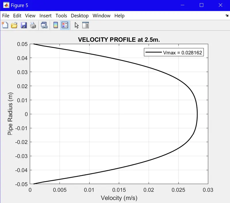
title('VELOCITY PROFILE at 2.5m.')

% Plot all the graphs
figure(6)
plot(U_mag_1,r_pt,'g','linewidth',1.5)
hold on
plot(U_mag_1,r_pt_negative,'g','linewidth',1.5)
hold on
plot(U_mag_2,r_pt,'r','linewidth',1.5)
hold on
plot(U_mag_2,r_pt_negative,'r','linewidth',1.5)
hold on
plot(U_mag_3,r_pt,'b','linewidth',1.5)
hold on
plot(U_mag_3,r_pt_negative,'b','linewidth',1.5)
hold on
plot(U_mag_4,r_pt,'y','linewidth',1.5)
hold on
plot(U_mag_4,r_pt_negative,'y','linewidth',1.5)
hold on
plot(U_mag_5,r_pt,'k','linewidth',1.5)
hold on
plot(U_mag_5,r_pt_negative,'k','linewidth',1.5)
ylabel('Pipe Radius (m)')
xlabel('Velocity (m/s)')
title('VELOCITY PROFILES')
legend('20','','15','','10','','5','','2.5','')

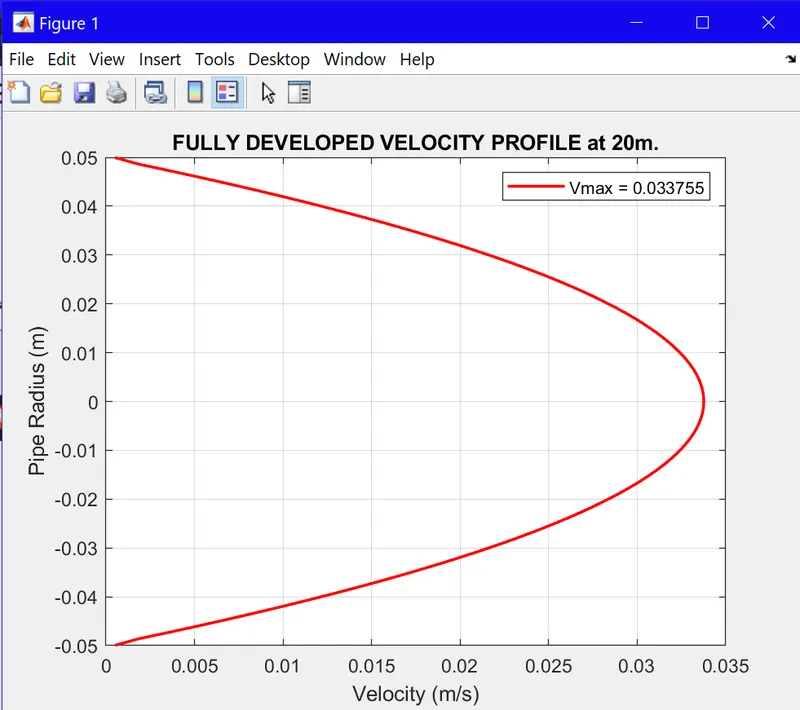
-->Computational results of Velocity Profiles at different lengths of the Pipe.

--> Maximum velocity as calculated is 0.033755 m/s. This is quite very to the analytical value of 0.0337 m/s obtained from the H-P equations.

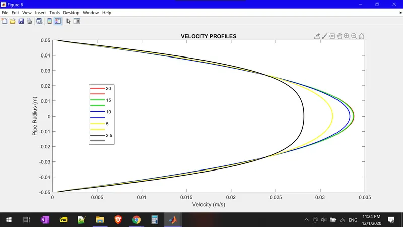
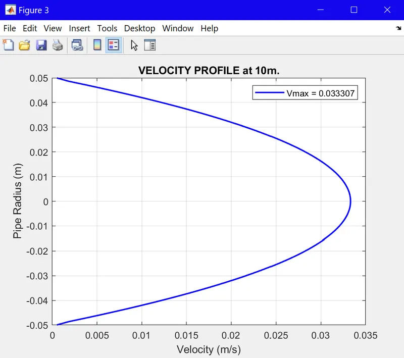
--> Following graphs shows the axis or centre-line velocity at (r=0). It shows us the variation of V max (maximum velocity) with the length of the Pipe. It also gives us an idea of Entrance length (Le), as at Entrance length it becomes stable and also attains maximum velocity(Vmax).

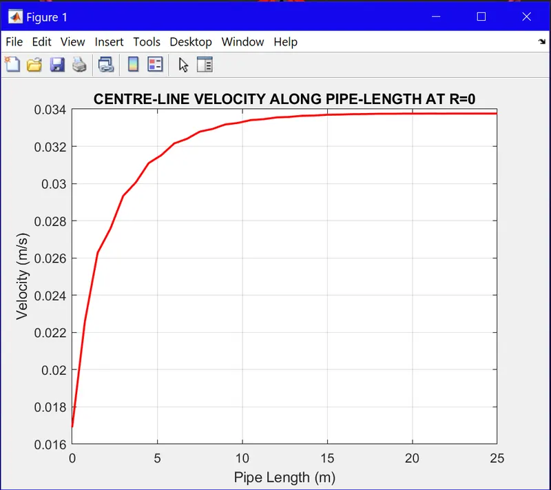
--> From the above graph we can see that Entrance Length is between [10-15] meters. This is quite accurate as we predicted 10 meters from H-P equations.

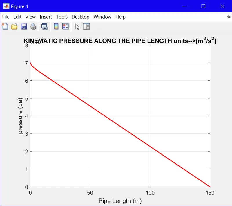
--> The next graph is the kinematic Pressure. The value of kinematic pressure drop is 0.007022 m. It is fairly accurate as we get 0.0068 m from the analytical H-P equations.

--> From this we can calculate absolute pressure drop by multiplying density with kinematic pressure. The absolute value is 7.000934 Pa, which is close to 6.7941 Pa obtained analytically.