Week 12 - Symmetry vs Wedge vs HP equation
wedge boundary condition vs symmetry boundary condition
--> In this project we have to compare the simulation results obtained for wedge and symmetry boundary conditions, compare and analyse them.
Wedge boundary conditions defines a axi-symmetric section of a cylinder and symmetry boundary condition defines a symmetric surface along which the geometry and the flow-field variables are mirrored.
--> Wedge is used for Axial and Spherical symmetry and there is a need to perform co-ordinate transformation for wedge angles which is different from just mirroring it (which happens in symmetry case).
--> Physical conditions are the same as previous challenge.
Diameter of the pipe -- D = 0.1 m = 10 cm
Reynold's Number -- Re = [D*v(avg)]/nu It must be less than 2100 for laminar flow (otherwise the flow will take transition to turbulance)
Working fluid --- Water at temperature 298 (degree kelvin).
Dynamic Viscosity --- mu = 8.4e-4 Pa.s
Density of Water --- rho = 997 Kg/m3
Kinematic Viscosity --- nu = 8.42527e-7 m2/s
Initial uniform velocity --- v = [nu*Re]/D ---> v = 0.0169 m/s
--- V(max) = 2*v = 0.0337 m/s
Entrance Length --- Le = 0.05*Re*D = 0.05*2000*0.1 = 10 m
Pressure drop △p --- △p= (32*mu*L*v)/(D)^2 = 6.7941 Pa
Kinematic Pressure drop --- △p(kinematic) = △p/rho = 0.0068 m
Shear stress --- τ = (4*mu*v)/r = 0.0011 Pa
--> Following is a MATLAB code for generating blockMeshDict file.(For symmetry boundary condition)
close all
clear all
clc
% Geometry of the pipe(Length and Diameter)
L=30;
d=0.1;
% Input Wedge Angle
thita=input("Enter the wedge angle--> ");
% Co-ordinates of the Wedge Section
x_pt= (d/2)*cosd(thita/2);
y_pt= (d/2)*sind(thita/2);
% Input scaling factors
sf_x=input("Enter the grading factor for x-axis--> ");
sf_y=input("Enter the grading factor for y-axis--> ");
sf_z=input("Enter the grading factor for z-axis--> ");
% Writing Strings for the BlockMeshDict File
foamFile = sprintf("FoamFile\n{\n    version    %s; \n    format     ascil; \n    class      dictionary; \n    object     blockMeshDict; \n}",'2.0');
scale = sprintf(" \nconvertToMeters  %d;",1);
vertices = sprintf("\nvertices\n(\n(0 0 0)\n(%d %d 0)\n(%d -%d 0)\n(0 0 %d)\n(%d %d %d)\n(%d -%d %d)\n);",x_pt,y_pt,x_pt,y_pt,L,x_pt,y_pt,L,x_pt,y_pt,L);
block = sprintf("\nblocks\n(\n    hex(0 2 1 0 3 5 4 3) (50 1 200) simpleGrading (%d %d %d)\n);",sf_x,sf_y,sf_z);
edge = sprintf("\nedges\n(\n    arc 1 2 (%d 0 0)\n    arc 4 5 (%d 0 %d)\n);",d/2,d/2,L);
boundary = sprintf("\nboundary\n(\n    inlet\n    {\n        type patch;\n        faces\n        (\n        (0 1 2 0)\n        );\n    }\n    outlet\n    {\n        type patch;\n        faces\n        (\n        (3 5 4 3)\n        );\n    }\n    tankWall\n    {\n        type wall;\n        faces\n        (\n        (1 4 5 2)\n        );\n    }\n    front\n    {\n        type symmetry;\n        faces\n        (\n        (0 3 4 1)\n        );\n    }\n    back\n    {\n        type symmetry;\n        faces\n        (\n        (0 2 5 3)\n        );\n    }\n    axis\n    {\n        type symmetry;\n        faces\n        (\n        (0 3 3 0)\n        );\n    }\n);");
merge = sprintf("\nmergePatchPairs\n(\n);");
% Combining all the above strings in single array.
blockMeshDictString = strcat(foamFile , scale , vertices , block , edge , boundary , merge);
% Generating blockMeshDict File.
file = fopen('blockMeshDict', 'w');
fprintf(file,'%s',blockMeshDictString);
fclose(file);
--> For wedge angle = 45 degree.
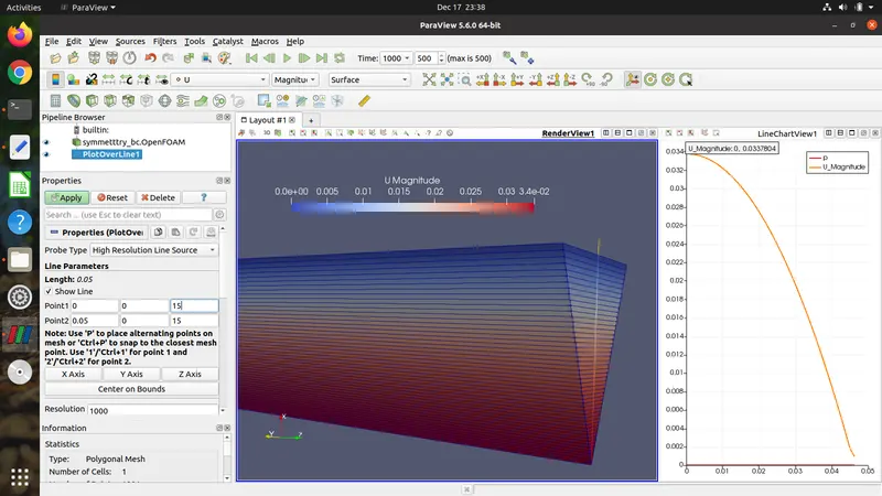
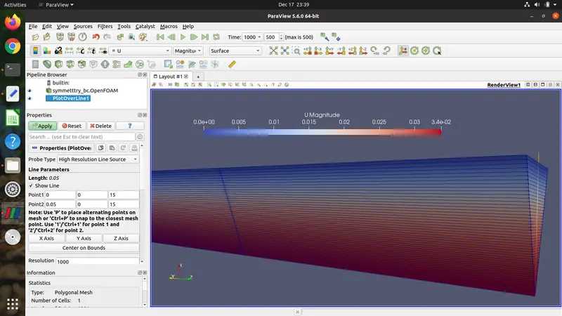
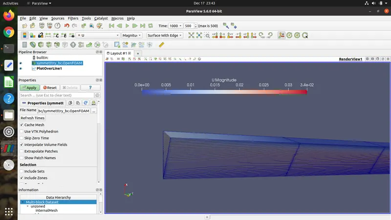
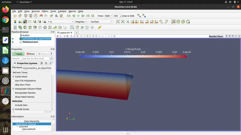
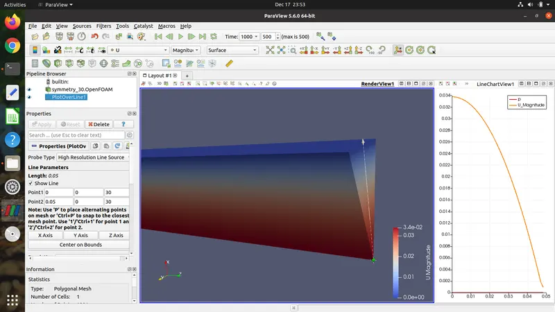
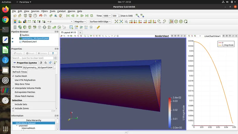
--> For wedge angle = 30 degrees.
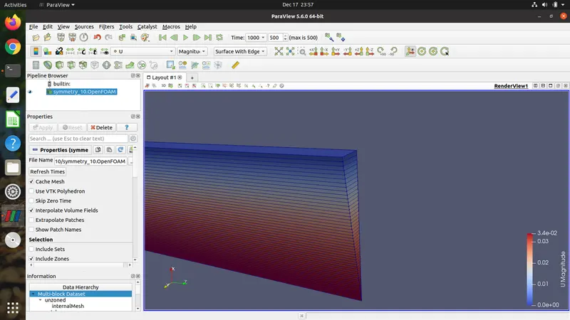
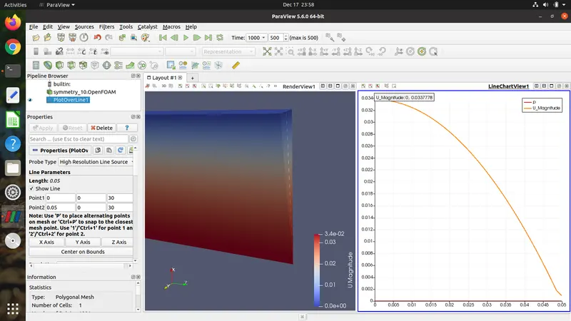
--> For wedge angle = 10 degrees.
Following MATLAB codes helps us to read the excell files generated after simulating the results.
clear all
close all
clc

% Plotting velocity profile for wedge boundary condition. (2 degrees)
V_x_1=xlsread('w21.csv','w21','A1:A1002'); % x-component of velocity
V_y_1=xlsread('w21.csv','w21','B1:B1002'); % y-component of velocity
V_z_1=xlsread('w21.csv','w21','C1:C1002'); % z-component of velocity
r_pt=xlsread('w21.csv','w21','G2:G1001'); % points along the radius
r_pt_negative= (-r_pt);
U_mag_1=(V_x_1.^2 + V_y_1.^2 + V_z_1.^2).^(1/2);
figure(1)
plot(U_mag_1,r_pt,'r','linewidth',1.5)
hold on
plot(U_mag_1,r_pt_negative,'r','linewidth',1.5)
grid on
ylabel('Pipe Radius (m)')
xlabel('Velocity (m/s)')

title('FULLY DEVELOPED VELOCITY PROFILE (WEDGE BC Thita = 2 degree)')

% Plotting velocity profile for wedge boundary condition. (3 degrees)
V_x_1=xlsread('w31.csv','w31','A1:A1002'); % x-component of velocity
V_y_1=xlsread('w31.csv','w31','B1:B1002'); % y-component of velocity
V_z_1=xlsread('w31.csv','w31','C1:C1002'); % z-component of velocity
r_pt=xlsread('w31.csv','w31','G2:G1001'); % points along the radius
r_pt_negative= (-r_pt);
U_mag_2=(V_x_1.^2 + V_y_1.^2 + V_z_1.^2).^(1/2);
figure(2)
plot(U_mag_2,r_pt,'r','linewidth',1.5)
hold on
plot(U_mag_2,r_pt_negative,'r','linewidth',1.5)
grid on
ylabel('Pipe Radius (m)')
xlabel('Velocity (m/s)')

title('FULLY DEVELOPED VELOCITY PROFILE (WEDGE BC Thita = 3 degree)')

% Plotting velocity profile for wedge boundary condition. (4 degrees)
V_x_1=xlsread('w41.csv','w41','A1:A1002'); % x-component of velocity
V_y_1=xlsread('w41.csv','w41','B1:B1002'); % y-component of velocity
V_z_1=xlsread('w41.csv','w41','C1:C1002'); % z-component of velocity
r_pt=xlsread('w41.csv','w41','G2:G1001'); % points along the radius
r_pt_negative= (-r_pt);
U_mag_3=(V_x_1.^2 + V_y_1.^2 + V_z_1.^2).^(1/2);
figure(3)
plot(U_mag_3,r_pt,'r','linewidth',1.5)
hold on
plot(U_mag_3,r_pt_negative,'r','linewidth',1.5)
grid on
ylabel('Pipe Radius (m)')
xlabel('Velocity (m/s)')

title('FULLY DEVELOPED VELOCITY PROFILE (WEDGE BC Thita = 4 degree)')


% Plotting velocity profile for wedge boundary condition. (5 degrees)
V_x_1=xlsread('w51.csv','w51','A1:A1002'); % x-component of velocity
V_y_1=xlsread('w51.csv','w51','B1:B1002'); % y-component of velocity
V_z_1=xlsread('w51.csv','w51','C1:C1002'); % z-component of velocity
r_pt=xlsread('w51.csv','w51','G2:G1001'); % points along the radius
r_pt_negative= (-r_pt);
U_mag_4=(V_x_1.^2 + V_y_1.^2 + V_z_1.^2).^(1/2);
figure(4)
plot(U_mag_4,r_pt,'r','linewidth',1.5)
hold on
plot(U_mag_4,r_pt_negative,'r','linewidth',1.5)
grid on
ylabel('Pipe Radius (m)')
xlabel('Velocity (m/s)')

title('FULLY DEVELOPED VELOCITY PROFILE (WEDGE BC Thita = 5 degree)')

% Plotting velocity profile for symmetry boundary condition (4 degree)
V_x_1=xlsread('s_4_1.csv','s_4_1','A1:A1002'); % x-component of velocity
V_y_1=xlsread('s_4_1.csv','s_4_1','B1:B1002'); % y-component of velocity
V_z_1=xlsread('s_4_1.csv','s_4_1','C1:C1002'); % z-component of velocity
r_pt=xlsread('s_4_1.csv','s_4_1','G2:G1001'); % points along the radius
r_pt_negative= (-r_pt);
U_mag_5=(V_x_1.^2 + V_y_1.^2 + V_z_1.^2).^(1/2);
figure(5)
plot(U_mag_5,r_pt,'r','linewidth',1.5)
hold on
plot(U_mag_5,r_pt_negative,'r','linewidth',1.5)
grid on
ylabel('Pipe Radius (m)')
xlabel('Velocity (m/s)')

title('FULLY DEVELOPED VELOCITY PROFILE SYMMETRY BC (Thita = 4 degree)')

% Plotting velocity profile for symmetry boundary condition (10 degree)
V_x_1=xlsread('s_10_1.csv','s_10_1','A1:A1002'); % x-component of velocity
V_y_1=xlsread('s_10_1.csv','s_10_1','B1:B1002'); % y-component of velocity
V_z_1=xlsread('s_10_1.csv','s_10_1','C1:C1002'); % z-component of velocity
r_pt=xlsread('s_10_1.csv','s_10_1','G1:G998'); % points along the radius
r_pt_negative= (-r_pt);
U_mag_6=(V_x_1.^2 + V_y_1.^2 + V_z_1.^2).^(1/2);
figure(6)
plot(U_mag_6,r_pt,'r','linewidth',1.5)
hold on
plot(U_mag_6,r_pt_negative,'r','linewidth',1.5)
grid on
ylabel('Pipe Radius (m)')
xlabel('Velocity (m/s)')

title('FULLY DEVELOPED VELOCITY PROFILE SYMMETRY BC (Thita = 10 degree)')

% Plotting velocity profile for symmetry boundary condition (30 degree)
V_x_1=xlsread('s_30_1.csv','s_30_1','A1:A1002'); % x-component of velocity
V_y_1=xlsread('s_30_1.csv','s_30_1','B1:B1002'); % y-component of velocity
V_z_1=xlsread('s_30_1.csv','s_30_1','C1:C1002'); % z-component of velocity
r_pt=xlsread('s_30_1.csv','s_30_1','G1:G967'); % points along the radius
r_pt_negative= (-r_pt);
U_mag_7=(V_x_1.^2 + V_y_1.^2 + V_z_1.^2).^(1/2);
figure(7)
plot(U_mag_7,r_pt,'r','linewidth',1.5)
hold on
plot(U_mag_7,r_pt_negative,'r','linewidth',1.5)
grid on
ylabel('Pipe Radius (m)')
xlabel('Velocity (m/s)')

title('FULLY DEVELOPED VELOCITY PROFILE SYMMETRY BC (Thita = 30 degree)')

% Plotting velocity profile for symmetry boundary condition (45 degree)
V_x_1=xlsread('s_45_1.csv','s_45_1','A1:A1002'); % x-component of velocity
V_y_1=xlsread('s_45_1.csv','s_45_1','B1:B1002'); % y-component of velocity
V_z_1=xlsread('s_45_1.csv','s_45_1','C1:C1002'); % z-component of velocity
r_pt_1=xlsread('s_45_1.csv','s_45_1','G2:G925'); % points along the radius
r_pt_negative_1= (-r_pt_1);
U_mag_8=(V_x_1.^2 + V_y_1.^2 + V_z_1.^2).^(1/2);
figure(8)
plot(U_mag_8,r_pt_1,'r','linewidth',1.5)
hold on
plot(U_mag_8,r_pt_negative_1,'r','linewidth',1.5)
grid on
ylabel('Pipe Radius (m)')
xlabel('Velocity (m/s)')

title('FULLY DEVELOPED VELOCITY PROFILE SYMMETRY BC (Thita = 45 degree)')
clear all
close all
clc

% Plotting velocity profile for wedge boundary condition. (2 degrees)
V_x_1=xlsread('w22.csv','w22','A1:A1002'); % x-component of velocity
V_y_1=xlsread('w22.csv','w22','B1:B1002'); % y-component of velocity
V_z_1=xlsread('w22.csv','w22','C1:C1002'); % z-component of velocity
r_pt=xlsread('w22.csv','w22','I1:I1002'); % points along the radius

U_mag_1=(V_x_1.^2 + V_y_1.^2 + V_z_1.^2).^(1/2);
figure(1)
plot(U_mag_1,r_pt,'r','linewidth',1.5)

grid on
ylabel('Pipe Radius (m)')
xlabel('Velocity (m/s)')
legend('Vmax = 0.033745')
title('AXIAL  VELOCITY PROFILE (WEDIE BC Thita = 2 degree)')

% Plotting velocity profile for wedge boundary condition. (3 degrees)
V_x_1=xlsread('w32.csv','w32','A1:A1002'); % x-component of velocity
V_y_1=xlsread('w32.csv','w32','B1:B1002'); % y-component of velocity
V_z_1=xlsread('w32.csv','w32','C1:C1002'); % z-component of velocity
r_pt=xlsread('w32.csv','w32','I1:I1002'); % points along the radius

U_mag_2=(V_x_1.^2 + V_y_1.^2 + V_z_1.^2).^(1/2);
figure(2)
plot(U_mag_2,r_pt,'r','linewidth',1.5)
grid on
ylabel('Pipe Radius (m)')
xlabel('Velocity (m/s)')

title('AXIAL  VELOCITY PROFILE (WEDIE BC Thita = 3 degree)')

% Plotting velocity profile for wedge boundary condition. (4 degrees)
V_x_1=xlsread('w42.csv','w42','A1:A1002'); % x-component of velocity
V_y_1=xlsread('w42.csv','w42','B1:B1002'); % y-component of velocity
V_z_1=xlsread('w42.csv','w42','C1:C1002'); % z-component of velocity
r_pt=xlsread('w42.csv','w42','I1:I1002'); % points along the radius

U_mag_3=(V_x_1.^2 + V_y_1.^2 + V_z_1.^2).^(1/2);
figure(3)
plot(U_mag_3,r_pt,'r','linewidth',1.5)
grid on
ylabel('Pipe Radius (m)')
xlabel('Velocity (m/s)')

title('AXIAL  VELOCITY PROFILE (WEDIE BC Thita = 4 degree)')


% Plotting velocity profile for wedge boundary condition. (5 degrees)
V_x_1=xlsread('w5222.csv','w5222','A1:A1002'); % x-component of velocity
V_y_1=xlsread('w5222.csv','w5222','B1:B1002'); % y-component of velocity
V_z_1=xlsread('w5222.csv','w5222','C1:C1002'); % z-component of velocity
r_pt=xlsread('w5222.csv','w5222','I1:I1002'); % points along the radius

U_mag_4=(V_x_1.^2 + V_y_1.^2 + V_z_1.^2).^(1/2);
figure(4)
plot(U_mag_4,r_pt,'r','linewidth',1.5)
grid on
ylabel('Pipe Radius (m)')
xlabel('Velocity (m/s)')

title('AXIAL  VELOCITY PROFILE (WEDIE BC Thita = 5 degree)')

% Plotting velocity profile for symmetry boundary condition (4 degree)
V_x_1=xlsread('s_4_2.csv','s_4_2','A1:A1002'); % x-component of velocity
V_y_1=xlsread('s_4_2.csv','s_4_2','B1:B1002'); % y-component of velocity
V_z_1=xlsread('s_4_2.csv','s_4_2','C1:C1002'); % z-component of velocity
r_pt=xlsread('s_4_2.csv','s_4_2','I1:I1002'); % points along the radius

U_mag_5=(V_x_1.^2 + V_y_1.^2 + V_z_1.^2).^(1/2);
figure(5)
plot(U_mag_5,r_pt,'r','linewidth',1.5)
grid on
ylabel('Pipe Radius (m)')
xlabel('Velocity (m/s)')

title('AXIAL  VELOCITY PROFILE SYMMETRY BC (Thita = 4 degree)')

% Plotting velocity profile for symmetry boundary condition (10 degree)
V_x_1=xlsread('s_10_2.csv','s_10_2','A1:A1002'); % x-component of velocity
V_y_1=xlsread('s_10_2.csv','s_10_2','B1:B1002'); % y-component of velocity
V_z_1=xlsread('s_10_2.csv','s_10_2','C1:C1002'); % z-component of velocity
r_pt=xlsread('s_10_2.csv','s_10_2','I1:I1002'); % points along the radius

U_mag_6=(V_x_1.^2 + V_y_1.^2 + V_z_1.^2).^(1/2);
figure(6)
plot(U_mag_6,r_pt,'r','linewidth',1.5)
grid on
ylabel('Pipe Radius (m)')
xlabel('Velocity (m/s)')

title('AXIAL  VELOCITY PROFILE SYMMETRY BC (Thita = 10 degree)')

% Plotting velocity profile for symmetry boundary condition (30 degree)
V_x_1=xlsread('s_30_2.csv','s_30_2','A1:A1002'); % x-component of velocity
V_y_1=xlsread('s_30_2.csv','s_30_2','B1:B1002'); % y-component of velocity
V_z_1=xlsread('s_30_2.csv','s_30_2','C1:C1002'); % z-component of velocity
r_pt=xlsread('s_30_2.csv','s_30_2','I1:I1002'); % points along the radius

U_mag_7=(V_x_1.^2 + V_y_1.^2 + V_z_1.^2).^(1/2);
figure(7)
plot(U_mag_7,r_pt,'r','linewidth',1.5)
grid on
ylabel('Pipe Radius (m)')
xlabel('Velocity (m/s)')

title('AXIAL  VELOCITY PROFILE SYMMETRY BC (Thita = 30 degree)')

% Plotting velocity profile for symmetry boundary condition (45 degree)
V_x_1=xlsread('s_45_2.csv','s_45_2','A1:A1002'); % x-component of velocity
V_y_1=xlsread('s_45_2.csv','s_45_2','B1:B1002'); % y-component of velocity
V_z_1=xlsread('s_45_2.csv','s_45_2','C1:C1002'); % z-component of velocity
r_pt_1=xlsread('s_45_2.csv','s_45_2','I1:I1002'); % points along the radius

U_mag_8=(V_x_1.^2 + V_y_1.^2 + V_z_1.^2).^(1/2);
figure(8)
plot(U_mag_8,r_pt_1,'r','linewidth',1.5)
grid on
ylabel('Pipe Radius (m)')
xlabel('Velocity (m/s)')

title('AXIAL VELOCITY PROFILE SYMMETRY BC (Thita = 45 degree)')
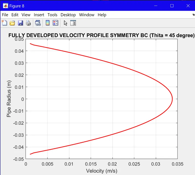
--> Velocity profile at wedge angle = 45 degree.(Symmetry BC)
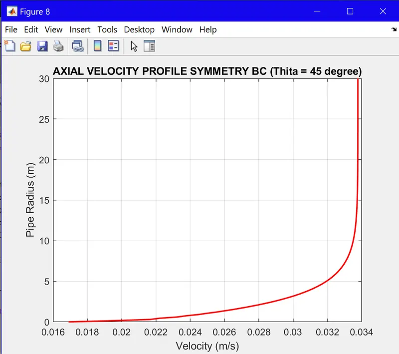
--> Centre-line axial velocity for wedge angle = 45 degrees.(Symmetry BC)
Following are the overall observations recorded in the table.
| WEDGE BOUNDARY CONDITION | WEDGE ANGLE (Degree) | V(max) H-P equations | V(max) Result | Clock Time (s) | % Error in V(max) | CFL (max) |
| 2 | 0.033700 | 0.0337777 | 968 | 0.2305 | 0.0129756 | |
| 3 | 0.033700 | 0.0337778 | 865 | 0.2308 | 0.012977 | |
| 4 | 0.033700 | 0.0337778 | 895 | 0.2308 | 0.0129791 | |
| 5 | 0.033700 | 0.0337778 | 1144 | 0.2308 | 0.0129817 | |
| SYMMETRY BOUNDARY CONDITION | WEDGE ANGLE (Degree) | V(max) H-P equations | V(max) Result | Clock Time (s) | % Error in V(max) | CFL (max) |
| 4 | 0.033700 | 0.0337235 | 1037 | 0.0697 | 0.0397189 | |
| 10 | 0.033700 | 0.0337778 | 852 | 0.2302 | 0.0397024 | |
| 30 | 0.033700 | 0.0337792 | 818 | 0.23501 | 0.0404545 | |
| 45 | 0.033700 | 0.0337804 | 941 | 0.2385 | 0.0415701 |
Conclusions :--
--> In a direct comparison of wedge vs symmetry (boundary condition) as shown above for 4 degrees wedge angle, symmetry BC has more accurate results (with less error) and takes more computational time than wedge BC.
--> Computational time depends on a no. of factors. We see an irregularity in clock time in the above results. The main contributing factors are Mesh Quality and number of cells in mesh. If cells in a mesh become skewed in shape then the quality of mesh is bad and simulation time is more. As the wedge angle increases number of cells increase in mesh which also contributes to more computational time.
--> For symmetry BC as wedge angle increases error in max. velocity also increases. As more computational units/cells contribute to more truncation error. For wedge BC max. velocity has very less variation as the wedge angle increases from 2 to 5 degree. In wedge BC we get minimum error for 2 degree wedge angle.