Week 7 - Simulation of a 1D Super-sonic nozzle flow simulation using Macormack Method
Simulation of a 1D Super-sonic nozzle flow simulation using MacCormack's Method
Aim: To simulate the isentropic flow through a quasi 1D subsonic-supersonic nozzle.
Objective:
To derive both the conservation and non-conservation forms of the governing equations and solve them using MacCormack's technique.
To determine the steady-state temperature distribution for the flow-field variables and investigate the difference between the two forms of governing equations by comparing their solutions.
Theory:
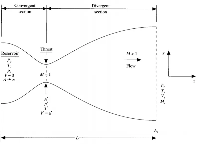
The isentropic flow through a quasi-1D subsonic-supersonic nozzle
The flow is locally subsonic in the convergent section of the nozzle, sonic at the throat (minimum area), and supersonic at the divergent section. The sonic flow (M=1)at the throat means the local velocity at this section is equal to the local speed of the sound.
`p_0,T_0` stagnation value
`p^star,T^star`sonic value at throat
`A^star`area at sonic throat
`P_e,V_e,T_e,M_e`exit value of pressure. velocity .temperature. and mach number`
flow expands isentropically to supersonic outlet
`(A/A^**)^2=1/M^2*(2/(gamma+1)*(1+(gamma-1)/2*M^2))^((gamma+1)/(gamma-1))`
`(p/p_o)=(1+(gamma-1)/2*M^2)^(-gamma/(gamma-1)`
`(rho/rho_o)=(1+(gamma-1)/2*M^2)^(-1/(gamma-1)`
`(T/T_o)=(1+(gamma-1)/2*M^2)^(-1)`
Mach number is a dimensionless quantity in fluid dynamics representing the ratio of flow velocity past a boundary to the local speed of sound.
`M=v/c`
where:
M is the local Mach number,
u is the local flow velocity with respect to the boundaries (either internal, such as an object immersed in the flow, or external, like a channel), and
c is the speed of sound in the medium, which in air varies with the square root of the thermodynamics temperature.
Assuming air to be an ideal gas, the formula to compute the Mach number in a subsonic compressible flow is derived from Bernoulli's equation for M < 1:
`M=sqrt(2/(gamma+1)*[(q_c/p+1)^((gamma-1)/(gamma))-1]`
and the speed of sound varies with temperature as follows:
`c=sqrt(gamma*R_**t)`
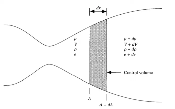
control volume for deriving the partial differential equation of isentropic flow through a quasi-1D subsonic-supersonic nozzle
We assume that at a given section, where the cross section area is A, the flow properties are uniform across the section. Hence, although the area of the nozzle changes as a function of distance along the nozzle, X, and therefore in reality the flow field is two-dimensional (the flow varies in the two-dimensional x-y space), We make the assumption that the flow properties vary only with X; this is tantamount to assuming uniform flow properties across any given cross-section. Such flow is defined as a Quasi-one-dimensional flow.
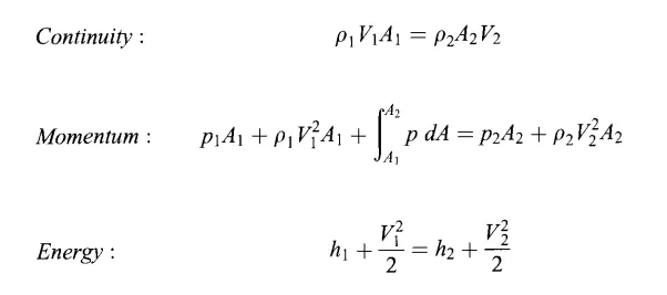
The governing continuity, momentum, and energy equations in terms of non-dimensional variables for this quasi-one-dimensional steady and isentropic flow can be expressed respectively as:
Non- Conservative :
Continuity equation:
`(delrho')/(delt') = -rho'((delv')/(delx')) - rho'v'((del(ln A'))/(delx')) - v'((delrho')/(delx'))`
Momentum equation:
`(delv')/(delt') = -v'((delv')/(delx')) -(1/gamma)((delt')/(delx') + (t')/(rho')((delrho')/(delx')))`
Energy equation:
`(delt')/(delt') = -v'((delt')/(delx')) - (gamma -1)t'[(delV')/(delx') + v'(del(lnA'))/(delx')]`
Conservative :
Continuity equation:
`(del(rho'A'))/(delt') + (del(rho'A'v'))/(delx') = 0`
Momentum equation:
`(del(rho'A'V'))/(delt') + (del[rho'A'(v')^2 +(1/gamma)rho'A'])/(delx') = (1/gamma)rho'((delA')/(delx'))`
Energy equation:
`(del[rho'((e')/(gamma-1) + (gamma/2)(v')^2)A'])/(delt') + (del[rho'((e')/(gamma-1) + (gamma/2)(v')^2)v'A' + rho'A'v'])/(delx') = 0`
`gamma=1.4`
solution vectors:`U_i`
flux vectors: `F_i`
source term: `J_2`
`U_1 = rho'A'`
`U_2 = rho'A'v'`
`U_3 = rho'[(T')/(gamma-1) + (gamma)/2 V'^2]A'`
`F_1 = rho'A'v' = U_2`
`F_2 = rho'A'v^2 + 1/(gamma) p'A' = (U_2^2)/(U_1) + (gamma-1)/(gamma) [U_3 - (gamma)/2 (U_2^2)/(U_1)]`
`F_3 = rho'((T')/(gamma-1) + (gamma)/2 v'^2)v'A' + p'A'v' = gamma (U_2U_3)/U_1 - (gamma(gamma-1))/2 (U_2^3)/(U_1^2)`
`J_2 = 1/(gamma) p' (delA')/(delx')`
After substituting these terms in governing equations, we have,
`(delU_1)/(delt') = - (delF_1)/(delx')`
`(delU_2)/(delt') = - (delF_2)/(delx') + J_2`
`(delU_3)/(delt') = - (delF_3)/(delx')`
The flow variables are calculated on the numerical solution of the above terms as,
`rho' = U_1/(A')`
`v' = (U_2)/(U_1)`
`T' = (gamma-1)[(U_3)/(U_1) - (gamma)/2 v'^2]`
`p' = rho'T'`
The initial conditions:
`rho'(t=0) = {(1.0,for 0<=x'<0.5),((1.0 - 0.366(x'-0.5)),for 0.5<=x'<1.5),((0.634 - 0.3879(x' - 1.5)),for 1.5<=x'<=3.5):}`
`T'(t=0) = {(1.0,for 0<=x'<0.5),((1.0 - 0.167(x'-0.5)),for 0.5<=x'<1.5),((0.833 - 0.3507(x' - 1.5)),for 1.5<=x'<=3.5):}`
`v'(t=0) = (U_2)/(rho'(t=0)A') = 0.59/(rho'(t=0)A')`considering a constant mass flow rate`
`U_2 = rho'A'V' = 0.59`
MacCormack method:
In computational fluid dynamics, the MacCormack method is a widely used discretization scheme for the numerical solution of hyperbolic partial differential equations.
MacCormack method provides second-order accuracy without the involvement of second-order derivative thus reducing the complexity of the calculation. It is an explicit method.
Setup followed to solve the 1D Super-sonic nozzle flow simulation using Macormack Method:-
1) The governing flow equations will be couched in terms of partial differential equations suitable for the time marching solution of quasi-one-dimensional flow
2) The finite-difference expressions pertaining to MacCormack's technique as applied to this problem will be set up.
To implement a finite-difference solution, we divide the x-axis along the nozzle into a number of discrete grid points,
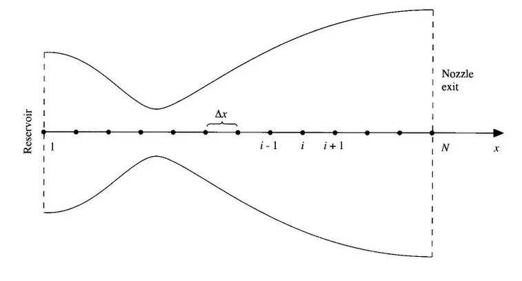
grid point distribution along the nozzle
The first grid point, labeled as point 1, is assumed to be in the reservoir. The points are evenly distributed along the x-axis, with △x">△x denoting the spacing between grid points. The last point, namely, that at the nozzle exit, is denoted by N; we have a total number of N grid points distributed along the axis. The point i is simply an arbitrary grid point, with points i-1 and i+1 as the adjacent points. MacCormack's technique is a predictor-corrector method. In the time marching approach, remember that we know the flow-field variables at time t, and we use the differential equations to solve explicitly for the variables at time t+△t">t+△t
3) Other details for the numerical solution (such as the calculation of timestep and the treatment of boundary conditions) will be formulated.
Non- Conservative :
Let f(x) is the equation to be solved. Then the following steps are followed:
- Initial profile
- predictor step
- solution update
- Corrector step
Conservative :
- Initializing of flux
- Predictor solution
- Solution update
- Updating primitive variable
- Corrector method
- Avg time derivative
- Final solution update
- Applying boundary conditions
The procedure of coding :
Code is started with clear all, close all, and clc to enable a fresh start without the manipulation of previous values.
Input parameters are assigned for the variables n, x, dx, n, gamma, A, nt .
Non-Conservative and Conservative forms functions are called ( created as Nonconservative_form and conservative_form).
Plotting is done for the following solutions
1. Steady-state distribution of primitive variables inside the nozzle
2. Time-wise variation of the primitive variables
3. Variation of Mass flow rate distribution inside the nozzle at different time steps during the time-marching process(inside the functions)
4. Comparison of Normalized mass flow rate distributions of both forms.
The procedure of creating functions:
- The purpose of the function is to calculate the values of Mass flow rate, Pressure, Mach number, Density, velocity, Temperature, Density at throat, velocity at throat, Temperature at throat, Mass flow rate at throat, Pressure at throat, Mach number at throat by the known equations for all the grid points.
- For this initial boundary conditions are established for Density, Temperature & Velocity and profiles for calculating area & throat.
- Now Outer Time loop is computed using for loop to calculate all the grid points for various formulas inside the loop.
- MacCormack technique is used to solve the numerical solution of governing equations such as Continuity, Momentum & Energy Equation.
- Predictor & Corrector methods are assigned within the for loop individually for calculating values.
- The calculated values are averaged in the next step and updating the solution with old values.
- Boundary Conditions are applied within the for loop and subsequently used for calculating the Mass Flow Rate, Mach Number & Pressure, and also calculating the values throat section.
- Finally plotting is done for Distance(x) & Mass Flow Rate for different timesteps(10,100,1000).
Main code:
close all
clear all
clc

%input parameters
n=31;
x=linspace(0,3,n);
dx=x(2)-x(1);
gamma=1.4;
A=1+2.2*(x-1.5).^2;
nt=1400;

% non conservative form
[m,p,M,rho,v,t,p_t,rho_t,v_t,t_t,M_t,m_t] = Nonconservative_form(n,nt);

% conservative form
[m_c,p_c,M_c,rho_c,v_c,t_c,p_tc,rho_tc,v_tc,t_tc,M_tc,m_tc] =conservative_form(n,nt);

%Steady state simulation for the primitive variables for Non-Conservative form
figure(3)
plot(x,rho,'color','r')
xlabel('x')
ylabel('density(rho)')
axis([0 3 0 1])
grid minor
title('x vs density(nonconservative)')
figure(4)
plot(x,v,'color','g')
xlabel('x')
ylabel('velocity(v)')
axis([0 3 0 1])
grid minor
title('x vs velocity(nonconservative)')
figure(5)
plot(x,t,'color','b')
xlabel('x')
ylabel('temperature(t)')
axis([0 3 0 1])
grid minor
title('x vs temperature(nonconservative)')
%Steady state simulation for the primitive variables for Conservative form
figure(6)
plot(x,rho_c,'color','r')
xlabel('x')
ylabel('density(rho)')
axis([0 3 0 1])
grid minor
title('x vs density(conservative)')
figure(7)
plot(x,v_c,'color','g')
xlabel('x')
ylabel('velocity(v_c)')
axis([0 3 0 1])
grid minor
title('x vs velocity(conservative)')
figure(8)
plot(x,t_c,'color','b')
xlabel('x')
ylabel('temperature(t_c)')
axis([0 3 0 1])
grid minor
title('x vs temperature(conservative)')

%Time-wise variation of the primitive variables at throat area for Non-Conservative and conservative form
nt=1:1400 ;
figure(9)
plot(nt,rho_t,'r',nt,rho_tc,'b')
xlabel('timestep(nt)')
ylabel('density(rho)')
title('Variation of density at nozzle throat')
legend('Non-Conservative','Conservative')
grid minor
figure(10)
plot(nt,v_t,'r',nt,v_tc,'b')
xlabel('timestep(nt)')
ylabel('velocity(v)')
title('Variation of velocity at nozzle throat')
legend('Non-Conservative','Conservative')
grid minor
figure(11)
plot(nt,t_t,'r',nt,t_tc,'b')
xlabel('timestep(nt)')
ylabel('temperature(t)')
title('Variation of Temperature at nozzle throat')
legend('Non-Conservative','Conservative')
grid minor

%Comparison of Normalized mass flow rate distributions of Non-Conservative and conservative forms
figure(12)
plot(x,m,'r',x,m_c,'b')
xlabel('x')
ylabel('mass flow rate')
title('Normalized mass flow rate at nozzle')
legend('Non-Conservative','Conservative')
grid minor
Function: Nonconservative_form
function [m,p,M,rho,v,t,p_t,rho_t,v_t,t_t,M_t,m_t] = Nonconservative_form(n,nt)
%inputs
x=linspace(0,3,n);
dx=x(2)-x(1);

%calculate initial profile
rho=1-0.3146*x;%density
t=1-0.2314*x;%temp
v=(0.1+1.09*x).*t.^0.5;%velocity
A=1+2.12*(x-1.5).^2;%area
gamma=1.4;%specific heat


%time steps

delta_t= 0.5*(dx./(sqrt(t)+v));
dt=min(delta_t);

%outer time loop
for k=1:nt
    delta_t= 0.5*(dx./(sqrt(t)+v));
    dt=min(delta_t);
    rho_old=rho;
    v_old=v;
    t_old=t;
    %predictor method
    %continuity equation
    for j=2:n-1
        %drho_dt_p(j)=-rho(j)*(v(j+1)-v(j))/dx-rho(j)*v(j)*(log(A(j+1))-log A(j))/dx-v(j)*(rho(j+1)-rho(j))/dx;
        dvdx=(v(j+1)-v(j))/dx;
        drhodx=(rho(j+1)-rho(j))/dx;
        dtdx=(t(j+1)-t(j))/dx;
        dlog_Adx=(log(A(j+1))-log(A(j)))/dx;
        drhodt_p(j)=-rho(j)*dvdx-rho(j)*v(j)*dlog_Adx-v(j)*drhodx;

        %monentum equation
        dvdt_p(j)=-v(j)*dvdx-(1/gamma)*(dtdx+(t(j)/rho(j))*drhodx);

        %energy equation
        dtdt_p(j)=-v(j)*dtdx-(gamma-1)*t(j)*(dvdx+v(j)*dlog_Adx);

        %solution update
        rho(j)=rho(j)+drhodt_p(j)*dt;
        v(j)=v(j)+dvdt_p(j)*dt;
        t(j)=t(j)+dtdt_p(j)*dt;
    end

    %corrector  method
    %continuity equation
    for j=2:n-1
        %drho_dt_p(j)=-rho(j)*(v(j)-v(j-1))/dx-rho(j)*v(j)*(log(A(j))-log A(j-1))/dx-v(j)*(rho(j)-rho(j-1))/dx;
        dvdx=(v(j)-v(j-1))/dx;
        drhodx=(rho(j)-rho(j-1))/dx;
        dtdx=(t(j)-t(j-1))/dx;
        dlog_Adx=(log(A(j))-log(A(j-1)))/dx;
        drhodt_c(j)=-rho(j)*dvdx-rho(j)*v(j)*dlog_Adx-v(j)*drhodx;
        %monentum equation
        dvdt_c(j)=-v(j)*dvdx-(1/gamma)*(dtdx+(t(j)/rho(j))*drhodx);
        %energy equation
        dtdt_c(j)=-v(j)*dtdx-(gamma-1)*t(j)*(dvdx+v(j)*dlog_Adx);

    end

    %avg time derivative

    drhodt_avg=0.5*(drhodt_p+drhodt_c);
    dvdt_avg=0.5*(dvdt_p+dvdt_c);
    dtdt_avg=0.5*(dtdt_p+dtdt_c);

    for i=2:n-1

        %final solution
        rho(i)=rho_old(i)+drhodt_avg(i)*dt;
        v(i)=v_old(i)+dvdt_avg(i)*dt;
        t(i)=t_old(i)+dtdt_avg(i)*dt;

    end

    %applying boundary condition

    %initial
    v(1)=2*v(2)-v(3);
    %outlet
    v(n)=2*v(n-1)-v(n-2);
    t(n)=2*t(n-1)-t(n-2);
    rho(n)=2*rho(n-1)-rho(n-2);

    %mach Number
    M = v./t.^0.5;

    %Pressure
    p = rho.*t;

    % mass flow rate
    m= rho.*v.*A;

    %throat = ((n-1)/2)+1
    throat = find(A==1);

    %Calculating Variables at throat section
    p_t(k)=p(throat);
    rho_t(k)=rho(throat) ;
    t_t(k)=t(throat);
    M_t(k)=M(throat);
    m_t(k)=m(throat);
    v_t(k)=v(throat);

    % mass flow rate plot
    figure(1)
    if  k==10
        plot (x,m,'r')
        hold on
    elseif k==100
        plot (x,m,'g')
        hold on
    elseif k==1000
        plot (x,m,'b')
        xlabel('x');
        ylabel('mass flow rate(m)');
        title('Variation of m at different time steps(Nonconservative)');
        legend('10','100','1000')
        grid minor

    end
end
Function: Conservative_form
function [m_c,p_c,M_c,rho_c,v_c,t_c,p_tc,rho_tc,v_tc,t_tc,M_tc,m_tc] =conservative_form(n,nt)

%inputs
x=linspace(0,3,n);
dx=x(2)-x(1);
A=1+2.12*(x-1.5).^2;%area
gamma=1.4;%specific heat

%calculate initial profile
%Desity and Temperature with respect to x
for i=1:length(x)
    if x(i)>=0 && x(i)<0.5
        rho_0(i) = 1;
        t_0(i) = 1;
    elseif x(i)>=0.5 && x(i)<1.5
        rho_0(i) = 1 - 0.366*(x(i)-0.5);
        t_0(i) = 1 - 0.167*(x(i)-0.5);
    elseif x(i)>=1.5 && x(i)<=3.5
        rho_0(i) = 0.634 - 0.3879*(x(i)-1.5);
        t_0(i) = 0.833 - 0.3507*(x(i)-1.5);
    end
    v_0(i) = 0.59/(rho_0(i)*A(i));
end

rho = rho_0;
t = t_0;
v = v_0;

%solution vector
U1 = rho.*A;
U2 = rho.*A.*v;
U3 = rho.*(t./(gamma-1) + 0.5*gamma*v.^2).*A;

%time steps
delta_t= 0.5*(dx./(sqrt(t)+v));
dt=min(delta_t);

%outer time loop
for k=1:nt
    delta_t= 0.5*(dx./(sqrt(t)+v));
    dt=min(delta_t);
    U1_old = U1;
    U2_old = U2;
    U3_old = U3;

    %intializing of flux
    for j=2:n-1
        F1 = U2;
        F2 = (U2.^2)./U1+((gamma-1)/gamma)*(U3 - 0.5*gamma*(U2.^2)./U1);
        F3 = gamma*U2.*U3./U1 - 0.5*gamma*(gamma-1)*(U2.^3)./(U1.^2);
        dF1dx = (F1(j+1) - F1(j))/dx;
        dF2dx = (F2(j+1) - F2(j))/dx;
        dF3dx = (F3(j+1) - F3(j))/dx;
        dAdx = (A(j+1) - A(j))/dx;
        J2 = (1/gamma)*rho(j)*t(j)*dAdx;

        % Predictor solution
        dU1dt_p(j) = -dF1dx;
        dU2dt_p(j) = -dF2dx + J2;
        dU3dt_p(j) = -dF3dx;

        %solution update
        U1(j) = U1(j) + dU1dt_p(j)*dt;
        U2(j) = U2(j) + dU2dt_p(j)*dt;
        U3(j) = U3(j) + dU3dt_p(j)*dt;

    end

    %updating premitive variable
    rho=U1./A;
    v = U2./U1;
    t = (gamma-1)*((U3./U1) - 0.5*gamma*v.^2);
    F1 = U2;
    F2 = (U2.^2)./U1+((gamma-1)/gamma)*(U3 - 0.5*gamma*(U2.^2)./U1);
    F3 = gamma*U2.*U3./U1 - 0.5*gamma*(gamma-1)*(U2.^3)./(U1.^2);

    %corrector  method
    for j=2:n-1
        dF1dx = (F1(j) - F1(j-1))/dx;
        dF2dx = (F2(j) - F2(j-1))/dx;
        dF3dx = (F3(j) - F3(j-1))/dx;
        dAdx = (A(j) - A(j-1))/dx;
        J2 = (1/gamma)*rho(j)*t(j)*dAdx;

        dU1dt_c(j) = -dF1dx;
        dU2dt_c(j) = -dF2dx + J2;
        dU3dt_c(j) = -dF3dx;
    end

    %avg time derivative
    dU1dt_avg = 0.5*(dU1dt_p + dU1dt_c);
    dU2dt_avg = 0.5*(dU2dt_p + dU2dt_c);
    dU3dt_avg = 0.5*(dU3dt_p + dU3dt_c);

    for i=2:n-1

        %final solution
        U1(i) = U1_old(i)+ dU1dt_avg(i)*dt;
        U2(i) = U2_old(i)+ dU2dt_avg(i)*dt;
        U3(i) = U3_old(i)+ dU3dt_avg(i)*dt;
    end

    %applying boundary condition
    %initial
    U1(1) = rho(1)*A(1);
    U2(1) = 2*U2(2) - U2(3);
    U3(1) = U1(1)*((t(1)/(gamma-1)) + 0.5*gamma*v(1)^2);
    %outlet
    U1(n) = 2*U1(n-1) - U1(n-2);
    U2(n) = 2*U2(n-1) - U2(n-2);
    U3(n) = 2*U3(n-1) - U3(n-2);

    %premitive variable
    rho = U1./A;
    v = U2./U1;
    t = (gamma-1)*((U3./U1) - 0.5*gamma*v.^2);

    %mach Number
    M = v./(t.^0.5);

    %Pressure
    p = rho.*t;

    % mass flow rate
    m = rho.*v.*A;

    %throat = ((n-1)/2)+1
    throat = find(A==1);

    %Calculating Variables at throat section
    p_t(k)=p(throat);
    rho_t(k)=rho(throat) ;
    t_t(k)=t(throat);
    M_t(k)=M(throat);
    m_t(k)=m(throat);
    v_t(k)=v(throat);

    m_c=m;
    p_c=p;
    M_c=M;
    rho_c=rho;
    v_c=v;
    t_c=t;
    p_tc=p_t;
    rho_tc= rho_t;
    v_tc= v_t;
    t_tc=t_t;
    M_tc= M_t;
    m_tc= m_t;

    % mass flow rate plot
    figure(2)
    if  k==10
        plot (x,m,'r')
        hold on
    elseif k==100
        plot (x,m,'g')
        hold on
    elseif k==1000
        plot (x,m,'b')
        xlabel('x');
        ylabel('mass flow rate(m)');
        title('Variation of m at different time steps(conservative)');
        legend('10','100','1000')
        grid minor

    end

end
Variation of Mass flow rate distribution inside the nozzle at different time steps during the time-marching process:
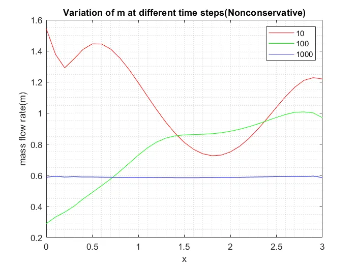
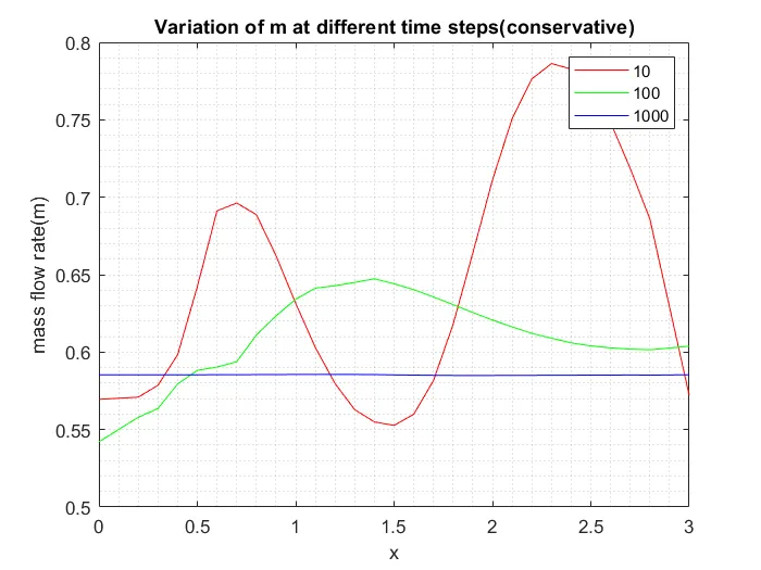
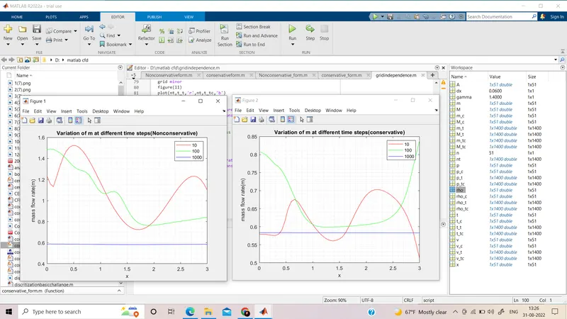
The above plots show that Mass Flow Rate at different time steps along the distance oscillates initially, however the solution becomes stable as we increase the number of timesteps.
Steady-state distribution of primitive variables inside the nozzle:
Primitive variables are density, velocity, and temperature.
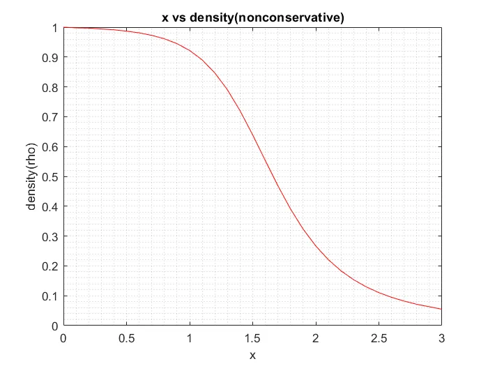
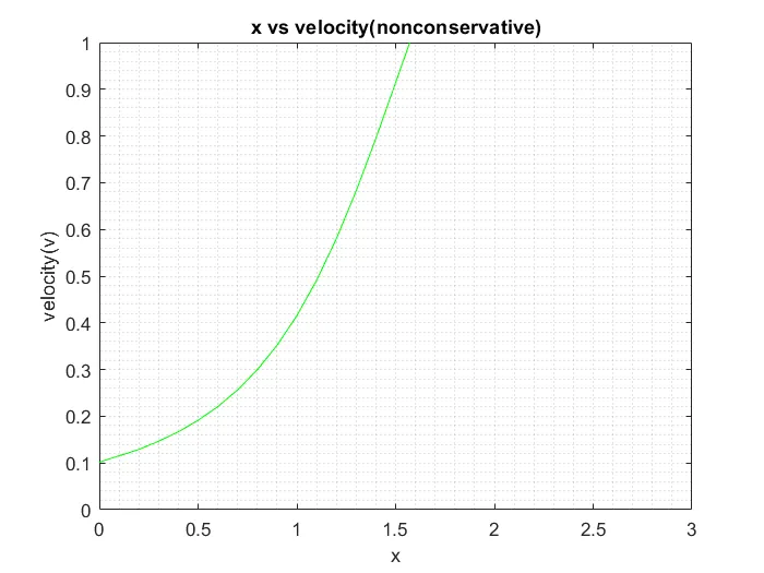
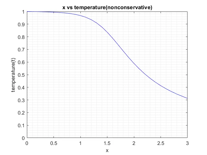
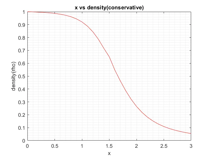
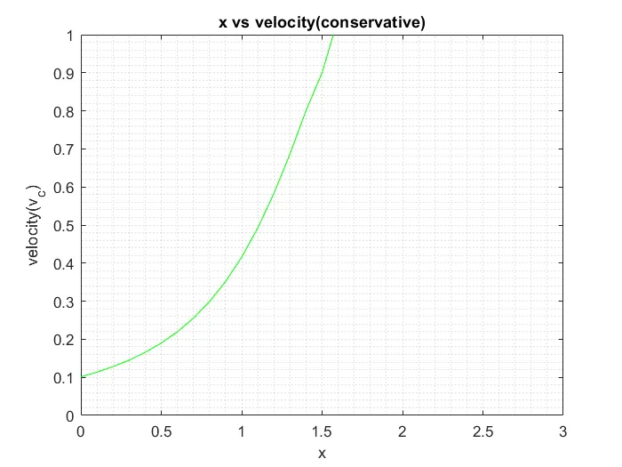
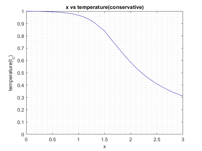
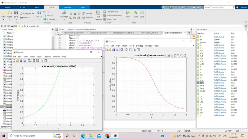
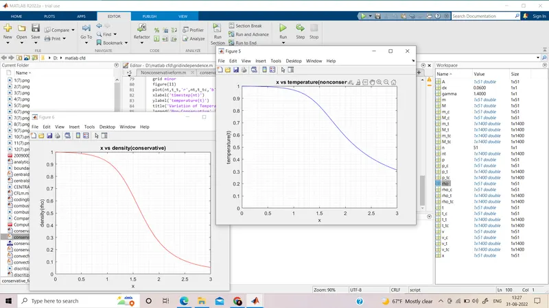
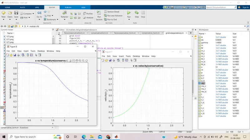
Here by observing the above plots we could see that both nonconservative and conservative forms are in the same phase giving the exact same solution for all the values.
Time-wise variation of the primitive variables:
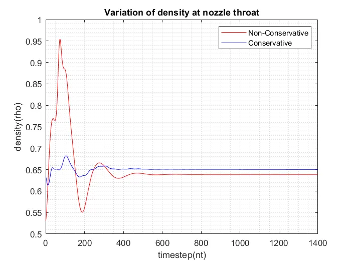
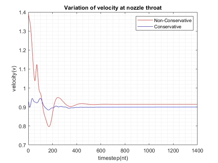
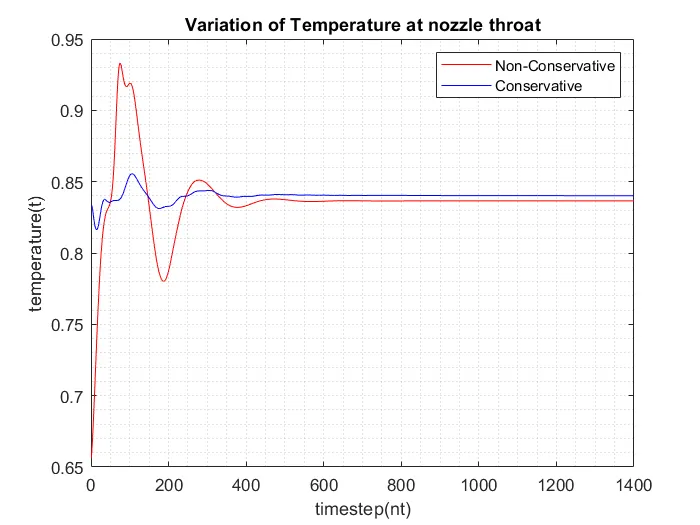
From the above plot, we can say:
At early times, the time derivatives are large and hence the values oscillated. These oscillations are associated with various unsteady compression and expansion waves which propagate through the nozzle during the transient process. At later times, the time derivatives rapidly grow small, changing by six orders of magnitude over a time span of 1400 time steps. Since we have used a finite no of time steps there will be some little amount of residual which is neglected. At the initial time steps, the Mach no. is not equal to 1 and after some time steps, it tends towards the value of 1 which represents the Converged solution. From the above profiles, we can clearly say that the minimum no of simulations for the solution to get into convergence is around 700~800 time steps. However, in order to get more accuracy, 1000 time steps would be ideal.
Comparison of Normalized mass flow rate distributions of both forms:
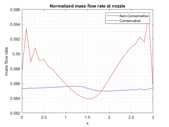
From the above plot, we can say that the conservation form gives a distribution that is much closer to being a constant. Whereas, the non-conservation form has a magnitude of a higher range with some surplus oscillations at both the inflow and outflow boundaries. The computational effort is much higher in the conservative form than in the non-conservative form. This is because it needs to decode the primitive variables from the flux variables. But such decoding is not necessary when solving non-conservative forms. So, based on the complexity, the time required to solve the conservation form is more than the non-conservation form.
Grid independence test on the solution :
In order to check if the solution is independent of the number of grid points used, a grid independence test was performed to ensure the solution's tenability. The number of grid divisions was increased to 50 (increasing grid points to 51) and the result is below:
close all
clear all
clc

%input parameters
n=51;
x=linspace(0,3,n);
dx=x(2)-x(1);
gamma=1.4;
A=1+2.2*(x-1.5).^2;
nt=1400;

% non conservative form
[m,p,M,rho,v,t,p_t,rho_t,v_t,t_t,M_t,m_t] = Nonconservative_form(n,nt);

% conservative form
[m_c,p_c,M_c,rho_c,v_c,t_c,p_tc,rho_tc,v_tc,t_tc,M_tc,m_tc] =conservative_form(n,nt);

%Steady state simulation for the primitive variables for Non-Conservative form
figure(3)
plot(x,rho,'color','r')
xlabel('x')
ylabel('density(rho)')
axis([0 3 0 1])
grid minor
title('x vs density(nonconservative)')
figure(4)
plot(x,v,'color','g')
xlabel('x')
ylabel('velocity(v)')
axis([0 3 0 1])
grid minor
title('x vs velocity(nonconservative)')
figure(5)
plot(x,t,'color','b')
xlabel('x')
ylabel('temperature(t)')
axis([0 3 0 1])
grid minor
title('x vs temperature(nonconservative)')
%Steady state simulation for the primitive variables for Conservative form
figure(6)
plot(x,rho_c,'color','r')
xlabel('x')
ylabel('density(rho)')
axis([0 3 0 1])
grid minor
title('x vs density(conservative)')
figure(7)
plot(x,v_c,'color','g')
xlabel('x')
ylabel('velocity(v_c)')
axis([0 3 0 1])
grid minor
title('x vs velocity(conservative)')
figure(8)
plot(x,t_c,'color','b')
xlabel('x')
ylabel('temperature(t_c)')
axis([0 3 0 1])
grid minor
title('x vs temperature(conservative)')

%Time-wise variation of the primitive variables at throat area for Non-Conservative and conservative form
nt=1:1400 ;
figure(9)
plot(nt,rho_t,'r',nt,rho_tc,'b')
xlabel('timestep(nt)')
ylabel('density(rho)')
title('Variation of density at nozzle throat')
legend('Non-Conservative','Conservative')
grid minor
figure(10)
plot(nt,v_t,'r',nt,v_tc,'b')
xlabel('timestep(nt)')
ylabel('velocity(v)')
title('Variation of velocity at nozzle throat')
legend('Non-Conservative','Conservative')
grid minor
figure(11)
plot(nt,t_t,'r',nt,t_tc,'b')
xlabel('timestep(nt)')
ylabel('temperature(t)')
title('Variation of Temperature at nozzle throat')
legend('Non-Conservative','Conservative')
grid minor

%Comparison of Normalized mass flow rate distributions of Non-Conservative and conservative forms
figure(12)
plot(x,m,'r',x,m_c,'b')
xlabel('x')
ylabel('mass flow rate')
title('Normalized mass flow rate at nozzle')
legend('Non-Conservative','Conservative')
grid minor
Changing grid point n=51
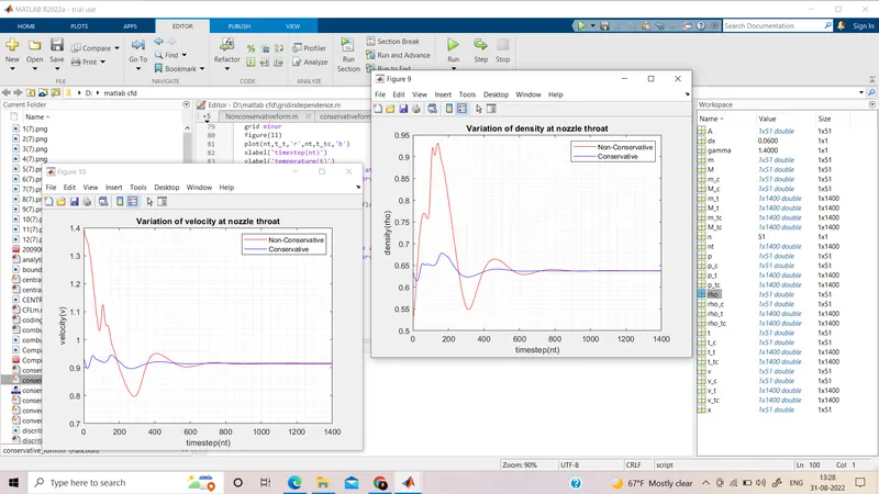
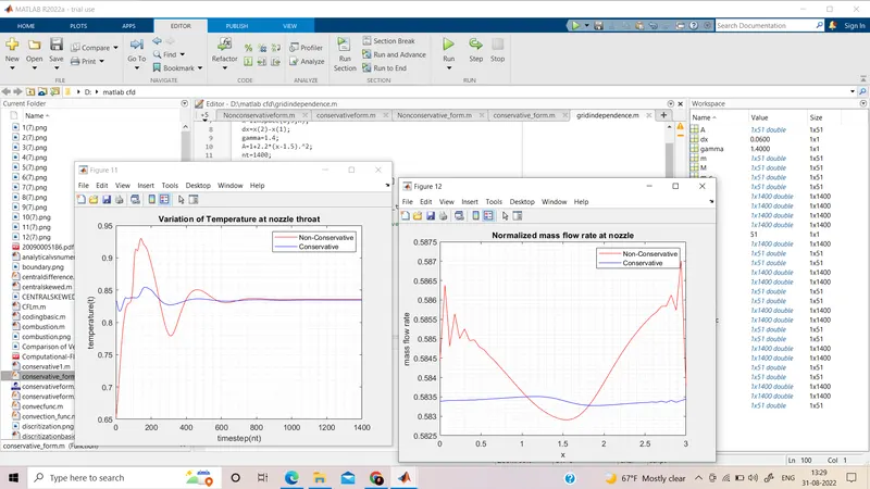
| n=31 at nt=1400 | n=51 at nt=1400 |
| rho=0.0546; rho_c=0.0545 | rho=0.0545 ;rho_c=0.0544 |
| v=1.8563;v_c=1.8563 | v=1.8571 ;v_c=1.8586 |
| t=0.3125 ; t_c=0.3097 | t=0.3121 ;t_c=0.3111 |
We can notice that the solution does not gain any significant improvement in precision when the number of grid points is increased. We can conclude from this that the solution is independent of the number of grid points used. If further precision is required for complex applications, the grid size can be increased accordingly.
Reference:CFD book by John Anderson