Week 7 - Simulation of a 1D Super-sonic nozzle flow simulation using Macormack Method
REPORT ON PROGRAM TO SIMULATE 1D QUASI SUBSONIC-SUPERSONIC NOZZLE
AIM
To Simulate the isentropic flow through a Quasi 1D subsonic nozzle by deriving both the conservation and non-conservation forms of the governing equations and solve them by implementing the MacCormack's technique using MATLAB.
Determine the steady-state temperature distribution for the flow-field variables and to investigate the difference between the two forms of governing equations by comparing their solutions along with the plots stated below.
- Steady-State distribution of primitive variable inside the nozzle.
- Time-wise variation of the primitive variable.
- Variation of Mass rate distribution inside the nozzle at different time steps during the time-marching process.
- Comparision of Normalized mass flow rate distributions of both forms.
THEORY
The isentropic flow through a quasi 1D subsonic-supersonic nozzle is shown in the below figure
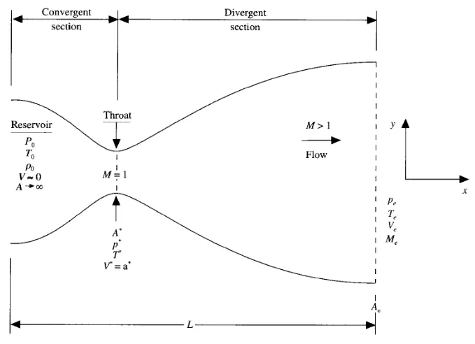
The above nozzle cosisits of two parts a convergent section and a divergent section which are termed as subsonic section and supersonic section respectively.
In the above figure we can see that the nozzle is subsonic at the entry, i.e the fluid enters into the nozzle throgh the subsonic/convergent area, where the mach number<1. Here the inlet temperature, pressure and density are denoted as P0, T0 and `rho0`. The velocity is approximated to 0, because the velocity at the inlet is the reservoir velocity which is around 0 m/s. The area at the inlet A is taken as infinity.
Then we have the throat section where the mach number M =1. At this point the area is the minimum and it is denoted as A*, pressure as p*, temperature as T* and the velocity V* is same as the speed of the sound a*. Then the exit section/supersonic section where the fluid exits at supersonic speed with mach number M>1. The temperature, pressure, velocity and mach number are denoted as `T_e,p_e,V_e and M_e`.
Here, we implement the numerical solution with Conservative and Non-Conservative forms.Governing Equations are marched in terms of PDE for both forms in order to use Time Marching solution for the problem. In the conservative and non conservative form we solve the Continuity, Momentum and Energy equations which actually calculates the required values of the fluid passing through the nozzle.
Conservative form:
In the Consevative form the control volume is fixed and the values at different grid points are calculated. Here the equation to calculate the continuity i.e rho is
`(del(rho'A'))/(delt')+(del(rho'A'V'))/(delx') = 0`
Momentum equation = `(del(rho'AV''))/(delt')+(del(rho'A'V'^2+(1/gamma)p'A'))/(delx') = (1/gamma)p'(delA')/(delx')`
Energy equation(T') = `(del(rho'((T')/(gamma-1)+(gamma/2)V'^2)A'))/(delt')+(del(rho'((T')/(gamma-1)+(gamma/2)V'^2)A'V'+rho'A'V'))/(delx') = 0`
Here we take rho'A' as U1 i.e U1 = `rho'A'` where U1 is the solution vector
U2 = `rho'A'V'`
U3 = `rho'((T')/(gamma-1)+(gamma/2)V'^2)A'`
Then we take spacial derivative terms and substitute it as flux terms, F1,F2 and F3
F1 = `rho'A'V'`
F2 = `rho'A'V'^2+(1/gamma)p'A'`
F3 = `rho'((T')/(gamma-1)+(gamma/2)V'^2)A'V'+rho'A'V'`
Then we have the source term at the momentum equation which we substitute as J2
J2 = `(1/gamma)p'(delA')/(delx')`
Non-Conservative form:
In the Non Consevative form the control volume is moving and we follow the fluid particles as they travel through the flow
Continuity equation(i.e time rate of change of density) = `(del(rho'A'))/(delt') + V'(del rho'A')/(delx') = -rho'A'(delV')/(delx')`
Momentum equation(i.e time rate of change of velocity) = `rho'(delV')/(delt')+rho'V'(delV')/(delx') = -(delp')/(delx')`
Energy equation(i.e rate of change of temperature) = `rho'(delT')/(delt')+rho'V'(delT')/(delx') = -p'(delV')/(delx')-p'V'(lnA)/(delx')`
This equation is converted into more suitable form which solves for the rate of change of density and we divide the continuity equation by A' which converts it into the form
Continuity equation = `(delrho')/(delt') = -rho'(delV')/(delx')-rho'V'(del(lnA'))/(delx')-V'(delrho')/(delx')`
Momentum equation = `(delV')/(delt') = -V'(delV')/(delt')-1/gamma((delT')/(delx')+(T')/(rho')(delrho')/(delx')`
Energy equation = `(delT')/(delt') = -V'(delT')/(delx')-(gamma-1)T'[(delV')/(delx')+V'(del(lnA'))/(delx')]`
In the above equations we use T',p',V',A',t' and x' in place of T,p,V,A,t and x because the former is dimensionless parameters because these equations used are required to be with no units,thus the equations are converted into the non dimensionalised form
x' = x/L L is the length of nozzle
p' = p/p0 p0 is the total pressure at inlet
V' = V/a0 a0 is the speed of sound
t' = t/L/a0
A' = A/A* A* is the throat area
Maccormack's Method :
Now we use Maccormack's method to calculate the solutions for conservative and non-conservative forms. For that the method is divided into two steps i.e the predictor and corrector step
At first we use the predictor step and solve the equation by using forward differencing for the space terms and then we update the solution using the equation
f* = `f_0+((delf)/(delt))_pDeltat`
Then the second step i.e the corrector step is carried out using backward differencing scheme for the space terms, here the updated f i.e f* is used in place of f, thus the equation turns out to be
`((delf^*)/(delt))_c`
Then the average of the corrector and predictor is found out and using this average value we calculate the actual value of f in the next time step i.e,
`((delf)/(delt))_(avg) = 0.5[((delf)/(delt))_p+((delf)/(delt))_c]`
`f^(n+1) = f_0+((delf)/(delt))Deltat`
`f_0`is the initial value.
BODY OF CONTENT
At first we define the function to find the solution using non-conservative method
function m_dot_non = func_non_conserve()
%inputs
nx = 31;
x = linspace(0,3,nx);
dx = x(2)-x(1);
gamma = 1.4;

%initial conditions
rho = 1-0.3146*x;
t0 = 1-0.2314*x;
v = (0.1+1.09*x).*(t0).^(0.5);
a = 1+2.2*(x-1.5).^2;
% r = 0.8314
sound = sqrt(t0)
c = 0.5;
%time steps
nt = 1400;
 dt1 = (c*dx)./(sound+v)
 dt = min(dt1)


%time loop
for k = 1:nt
    rho_old = rho;
    t0_old = t0;
    v_old = v;


    %predictor mathod

    for j =2:nx-1
        dvdx = (v(j+1)-v(j))/dx;
        dlogadx = (log(a(j+1))-log(a(j)))/dx;
        drhodx = (rho(j+1)-rho(j))/dx;
        dt0dx = (t0(j+1)-t0(j))/dx;
        %continuity equation
        drho_dt_p(j) = -rho(j)*dvdx-rho(j)*v(j)*dlogadx-v(j)*drhodx;
        %momentum equation
        dv_dt_p(j) = -v(j)*dvdx-(1/gamma)*(dt0dx+(t0(j)/rho(j))*drhodx);
        %energy equation
        dt0_dt_p(j) = -v(j)*dt0dx-(gamma-1)*t0(j)*(dvdx+v(j)*dlogadx);

        %solution update
        rho(j) = rho_old(j)+drho_dt_p(j)*dt;
        v(j) = v_old(j)+ dv_dt_p(j)*dt;
        t0(j) = t0_old(j)+ dt0_dt_p(j)*dt;
    end

        %corrector mathod
    for j =2:nx-1
        dvdx = (v(j)-v(j-1))/dx;
        dlogadx = (log(a(j))-log(a(j-1)))/dx;
        drhodx = (rho(j)-rho(j-1))/dx;
        dt0dx = (t0(j)-t0(j-1))/dx;
        %continuity equation
        drho_dt_c(j) = -rho(j)*dvdx-rho(j)*v(j)*dlogadx-v(j)*drhodx;
        %momentum equation
        dv_dt_c(j) = -v(j)*dvdx-(1/gamma)*(dt0dx+(t0(j)/rho(j))*drhodx);
        %energy equation
        dt0_dt_c(j) = -v(j)*dt0dx-(gamma-1)*t0(j)*(dvdx+v(j)*dlogadx);


    end

%average time update
drho_dt_avg = 0.5*(drho_dt_p+drho_dt_c);
dv_dt_avg = 0.5*(dv_dt_p+dv_dt_c);
dt0_dt_avg = 0.5*(dt0_dt_p+dt0_dt_c);
  %solution update
  for i = 2:nx-1
        rho(i) = rho_old(i)+drho_dt_avg(i)*dt;
        v(i) = v_old(i)+dv_dt_avg(i)*dt;
        t0(i) = t0_old(i)+dt0_dt_avg(i)*dt;
  end

  %boundary condition

  %initial condition
  v(1) = 2*v(2)-v(3);
  rho(1) = 1;
  t0(1) = 1;

  %final condition
  v(nx) = 2*v(nx-1)-v(nx-2);
  rho(nx) = 2*rho(nx-1)-rho(nx-2);
  t0(nx) = 2*t0(nx-1)-t0(nx-2);

% plotting
figure(1)
   subplot(3,1,1)
   plot(x,v)
   xlabel('x')
   ylabel('v')
   title('Primitive variables against x in the non-conservative form')

   subplot(3,1,2)
   plot(x,rho)
   xlabel('x')
   ylabel('rho')

   subplot(3,1,3)
   plot(x,t0)
   xlabel('x')
   ylabel('t0')


   pause(0.03)
  rho_throat(k) = rho(16);
  v_throat(k) = v(16);
  t0_throat(k) = t0(16);

   m_dot_non = rho.*a.*v;
    if (k==100)
     figure(2)
     plot(x,m_dot_non)
     hold on
    elseif (k==200)
     figure(2)
     plot(x,m_dot_non)
    elseif (k==500)
     figure(2)
     plot(x,m_dot_non)
    elseif (k==700)
     figure(2)
     plot(x,m_dot_non)
     xlabel('x')
     ylabel('m_dot-non')
     legend('k==100','k==200','k==500','k==700')
     title('Mass flow rate at varying time steps for non conservative')
    end


end
  m = v./sqrt(t0);
  figure(3)
  plot(x,m)
  xlabel('x')
  ylabel('mach number')
  title('mach number vs x using non-conservative method ')

    figure(4)
 subplot(3,1,1)
 plot(rho_throat)
 xlabel('time steps')
 ylabel('rho')
 title(' Primitive variables at throat vs Time steps')
 subplot(3,1,2)
 plot(v_throat)
 xlabel('time steps')
 ylabel('velocity')

 subplot(3,1,3)
 plot(t0_throat)
 xlabel('time steps')
 ylabel('Temperature')

end
In the above function first we input the values and initial conditions like density, temperature, velocity, area of the nozzle, speed of sound and courant number and then we input the time step and dt which is the minimum value of all the dt values calculated using the equation c*dx/sound+v
Now we start the time loop which varies from 1 to nt and inside the time loop first we store the values of rho, t0 and v as rho_old, t0_old and v_old.
Then as discussed we start solving the solution with the predictor method, for that first we create a for loop 'j' which varies from 2 to nx-1 and inside the loop we assign the values of(v(j+1)-v(j))/dx,(log(a(j+1))-log(a(j)))/dx, (rho(j+1)-rho(j))/dx, (t0(j+1)-t0(j))/dx as shown below
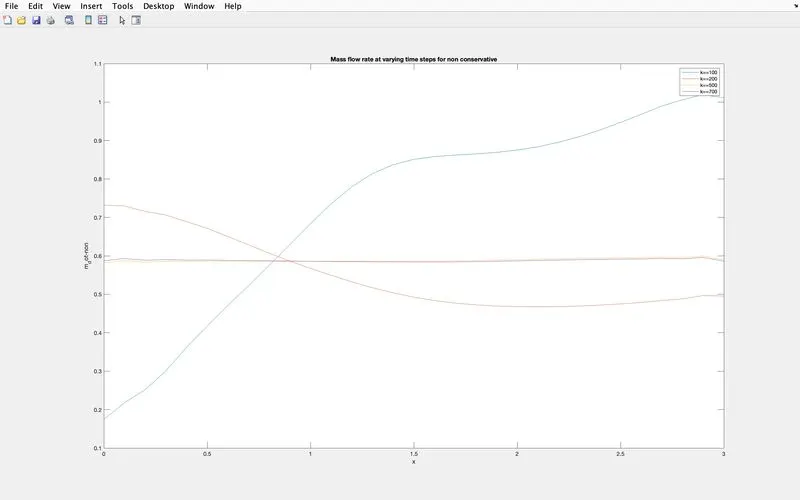
and plot it for differnt time steps(here time step k is given a values of 100,200,500 and 700) using an if condition.
function m_dot_con = conv_func()
%inputs
nx = 31;
x = linspace(0,3,nx);
dx = x(2)-x(1);
gamma = 1.4;
c = 0.5
%time steps
nt = 1400;


%initial conditions
for i =1:nx
    if(x(i)>=0) && (x(i)<=0.5)
        rho(i) = 1;
        t0(i) = 1;

    elseif(x(i)>=0.5) && (x(i)<=1.5)
        rho(i) = 1-0.366*(x(i)-0.5);
        t0(i) = 1-0.167*(x(i)-0.5);
    elseif(x(i)>=1.5) && (x(i)<=3)
        rho(i) = 0.634-0.3879*(x(i)-1.5);
        t0(i) = 0.833-0.3507*(x(i)-1.5);
    end
end

a = 1+2.2*(x-1.5).^2;
v = 0.59./(rho.*a);
sound = sqrt(t0);
%solution vector
u1 = rho.*a;
u2 = rho.*a.*v;
u3 = rho.*((t0./(gamma-1))+(gamma/2)*v.^2).*a;

for k = 1:nt
    dt1 = (c*dx)./(sound+v);
    dt = min(dt1);
    u1old = u1;
    u2old = u2;
    u3old = u3;

    f1 = u2;
    f2 = (u2.^2./u1)+((gamma-1)/gamma)*(u3-(gamma/2)*(u2.^2)./u1);
    f3 = gamma*((u2.*u3)./u1)-gamma*(gamma-1)/2*(u2.^3./u1.^2);


    %predictor method
    for i = 2:nx-1
        %continuity equation
        du1_dt_p(i) = -(f1(i+1)-f1(i))/dx;
        %momentum equation
        du2_dt_p(i) = -((f2(i+1)-f2(i))/dx)+(1/gamma)*rho(i)*t0(i)*((a(i+1)-a(i))/dx);
        %energy equation
        du3_dt_p(i) = -(f3(i+1)-f3(i))/dx;

        %solution update
        u1(i) = u1old(i)+du1_dt_p(i)*dt;
        u2(i) = u2old(i)+du2_dt_p(i)*dt;
        u3(i) = u3old(i)+du3_dt_p(i)*dt;


    end

        rho = u1./a;
        v =u2./u1;
        t0 = (gamma-1)*((u3./u1)-(gamma/2)*v.^2);
        p = rho.*t0;
      %flux values update
        f1 = u2;
        f2 = (u2.^2./u1)+((gamma-1)/gamma)*(u3-(gamma/2)*(u2.^2)./u1);
        f3 = gamma*((u2.*u3)./u1)-gamma*(gamma-1)/2*(u2.^3./u1.^2);

    %corrector step
    for i = 2:nx-1
        %continuity equation
        du1_dt_c(i) = -(f1(i)-f1(i-1))/dx;
        %momentum equation
        du2_dt_c(i) = -((f2(i)-f2(i-1))/dx)+(1/gamma)*rho(i)*t0(i)*((a(i)-a(i-1))/dx);
        %energy equation
        du3_dt_c(i) = -(f3(i)-f3(i-1))/dx;


    end
    %average time update
    du1_dt_avg = 0.5*(du1_dt_c+du1_dt_p);
    du2_dt_avg = 0.5*(du2_dt_c+du2_dt_p);
    du3_dt_avg = 0.5*(du3_dt_c+du3_dt_p);

    %final solution update
    for i = 2:nx-1
        u1(i) = u1old(i)+(du1_dt_avg(i))*dt;
        u2(i) = u2old(i)+(du2_dt_avg(i))*dt;
        u3(i) = u3old(i)+(du3_dt_avg(i))*dt;
    end

    %initial conditions
    u1(1) = rho(1)*a(1);
    u2(1) = 2*u2(2)-u2(3);
    u3(1) = u1(1)*((t0(1)/(gamma-1))+(gamma/2)*v(1)^2);

    % boundary condtions
    u1(nx) = 2*u1(nx-1)-u1(nx-2);
    u2(nx) = 2*u2(nx-1)-u2(nx-2);
    u3(nx) = 2*u3(nx-1)-u3(nx-2);

    %primitive variables
    rho = u1./a;
    v =u2./u1;
    t0 = (gamma-1)*((u3./u1)-(gamma/2)*v.^2);
    p = rho.*t0;


    %plotting
    figure(5)
    subplot(3,1,1)
    plot(x,rho)
    xlabel('x')
    ylabel('rho')
    title('Primitive variables against x in the conservative form')

    subplot(3,1,2)
    plot(x,v)
    xlabel('x')
    ylabel('v')
    subplot(3,1,3)
    plot(x,t0)
    xlabel('x')
    ylabel('t0')

    pause(0.03)

    u1_throat(k) = u1(16);
    u2_throat(k) = u2(16);
    u3_throat(k) = u3(16);
    m_dot_con = rho.*a.*v;
    if (k==100)
        figure(6)
     plot(x,m_dot_con)
     hold on
    elseif (k==200)
         figure(6)
      plot(x,m_dot_con)
     elseif (k==500)
         figure(6)
      plot(x,m_dot_con)
     elseif (k==700)
         figure(6)
     plot(x,m_dot_con)
     xlabel('x')
     ylabel('m_dot_con')
     legend('k==100','k==200','k==500','k==700')
     title('Mass flow rate at varying time steps for conservative form')

    end

end
%mach number
m = v./sqrt(t0);
figure(7)
plot(x,m)
xlabel('x')
ylabel('mach number')
 title('mach number vs x using conservative method ')
%plotting
figure(8)
subplot(3,1,1)
plot(u1_throat)
xlabel('number of time steps')
ylabel('u1_throat')
title(' Solution variables at throat vs Time steps')
subplot(3,1,2)
plot(u2_throat)
xlabel('number of time steps')
ylabel('u2_throat')
subplot(3,1,3)
plot(u3_throat)
xlabel('number of time steps')
ylabel('u3_throat')


end
In the above function also we input the same values, velocity, area of the nozzle, speed of sound and courant number and then we input the time step and dt which is the minimum value of all the dt values calculated using the equation c*dx/sound+v.
Here the initial condition is that as the length of the nozzle varies the density and temperature also varies. It is varied as shown below
and plot it for differnt time steps(here time step k is given a values of 100,200,500 and 700) using an if condition.
clear all
close all
clc


%calling function
m_dot_non = func_non_conserve()
m_dot_con = conv_func()
nx = 31
x = linspace(0,3,nx)
%plotting
figure(9)
plot(x,m_dot_con)
hold on
plot(x,m_dot_non)
xlabel('number of grids')
ylabel('mass flow rate')
title('comparison of the mass flow rates')
legend('conservative mass flow rate','non-conservative mass flow rate')
here we call the functions func_non_conserve and conv_func and store it as m_dot_non and m_dot_con.
Then we input the nx and x values which required for plotting purpose.
Now we jump into plotting where we plot the mass flow rate using convective method and mass flow rate using non-convective method and compare them by plotting them in a single plot of mass flow rate against x.
Then we label them using the label comand and give the suitable title using title command
function m_dot_non = func_non_conserve()
%inputs
nx = 31;
x = linspace(0,3,nx);
dx = x(2)-x(1);
gamma = 1.4;

%initial conditions
rho = 1-0.3146*x;
t0 = 1-0.2314*x;
v = (0.1+1.09*x).*(t0).^(0.5);
a = 1+2.2*(x-1.5).^2;
% r = 0.8314
sound = sqrt(t0)
c = 0.5;
%time steps
nt = 1400;
 dt1 = (c*dx)./(sound+v)
 dt = min(dt1)


%time loop
for k = 1:nt
    rho_old = rho;
    t0_old = t0;
    v_old = v;


    %predictor mathod

    for j =2:nx-1
        dvdx = (v(j+1)-v(j))/dx;
        dlogadx = (log(a(j+1))-log(a(j)))/dx;
        drhodx = (rho(j+1)-rho(j))/dx;
        dt0dx = (t0(j+1)-t0(j))/dx;
        %continuity equation
        drho_dt_p(j) = -rho(j)*dvdx-rho(j)*v(j)*dlogadx-v(j)*drhodx;
        %momentum equation
        dv_dt_p(j) = -v(j)*dvdx-(1/gamma)*(dt0dx+(t0(j)/rho(j))*drhodx);
        %energy equation
        dt0_dt_p(j) = -v(j)*dt0dx-(gamma-1)*t0(j)*(dvdx+v(j)*dlogadx);

        %solution update
        rho(j) = rho_old(j)+drho_dt_p(j)*dt;
        v(j) = v_old(j)+ dv_dt_p(j)*dt;
        t0(j) = t0_old(j)+ dt0_dt_p(j)*dt;
    end

        %corrector mathod
    for j =2:nx-1
        dvdx = (v(j)-v(j-1))/dx;
        dlogadx = (log(a(j))-log(a(j-1)))/dx;
        drhodx = (rho(j)-rho(j-1))/dx;
        dt0dx = (t0(j)-t0(j-1))/dx;
        %continuity equation
        drho_dt_c(j) = -rho(j)*dvdx-rho(j)*v(j)*dlogadx-v(j)*drhodx;
        %momentum equation
        dv_dt_c(j) = -v(j)*dvdx-(1/gamma)*(dt0dx+(t0(j)/rho(j))*drhodx);
        %energy equation
        dt0_dt_c(j) = -v(j)*dt0dx-(gamma-1)*t0(j)*(dvdx+v(j)*dlogadx);


    end

%average time update
drho_dt_avg = 0.5*(drho_dt_p+drho_dt_c);
dv_dt_avg = 0.5*(dv_dt_p+dv_dt_c);
dt0_dt_avg = 0.5*(dt0_dt_p+dt0_dt_c);
  %solution update
  for i = 2:nx-1
        rho(i) = rho_old(i)+drho_dt_avg(i)*dt;
        v(i) = v_old(i)+dv_dt_avg(i)*dt;
        t0(i) = t0_old(i)+dt0_dt_avg(i)*dt;
  end

  %boundary condition

  %initial condition
  v(1) = 2*v(2)-v(3);
  rho(1) = 1;
  t0(1) = 1;

  %final condition
  v(nx) = 2*v(nx-1)-v(nx-2);
  rho(nx) = 2*rho(nx-1)-rho(nx-2);
  t0(nx) = 2*t0(nx-1)-t0(nx-2);

% plotting
figure(1)
   subplot(3,1,1)
   plot(x,v)
   xlabel('x')
   ylabel('v')
   title('Primitive variables against x in the non-conservative form')

   subplot(3,1,2)
   plot(x,rho)
   xlabel('x')
   ylabel('rho')

   subplot(3,1,3)
   plot(x,t0)
   xlabel('x')
   ylabel('t0')


   pause(0.03)
  rho_throat(k) = rho(16);
  v_throat(k) = v(16);
  t0_throat(k) = t0(16);

   m_dot_non = rho.*a.*v;
    if (k==100)
     figure(2)
     plot(x,m_dot_non)
     hold on
    elseif (k==200)
     figure(2)
     plot(x,m_dot_non)
    elseif (k==500)
     figure(2)
     plot(x,m_dot_non)
    elseif (k==700)
     figure(2)
     plot(x,m_dot_non)
     xlabel('x')
     ylabel('m_dot-non')
     legend('k==100','k==200','k==500','k==700')
     title('Mass flow rate at varying time steps for non conservative')
    end


end
  m = v./sqrt(t0);
  figure(3)
  plot(x,m)
  xlabel('x')
  ylabel('mach number')
  title('mach number vs x using non-conservative method ')

    figure(4)
 subplot(3,1,1)
 plot(rho_throat)
 xlabel('time steps')
 ylabel('rho')
 title(' Primitive variables at throat vs Time steps')
 subplot(3,1,2)
 plot(v_throat)
 xlabel('time steps')
 ylabel('velocity')

 subplot(3,1,3)
 plot(t0_throat)
 xlabel('time steps')
 ylabel('Temperature')

end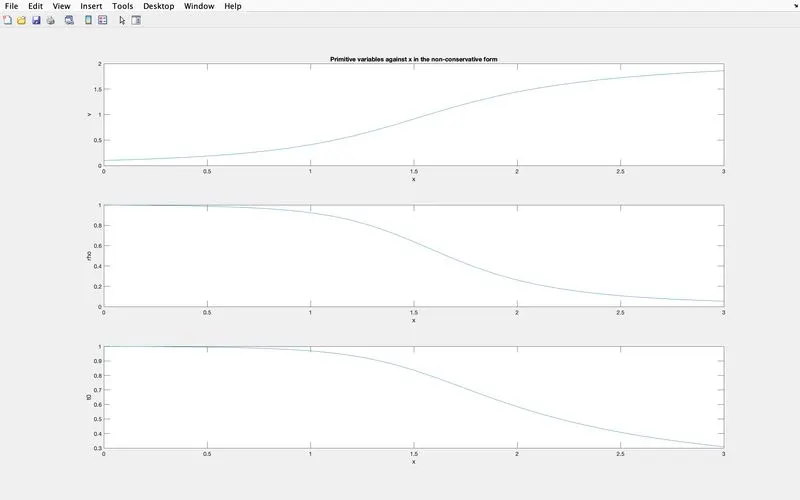
INFERENCE
In the above plot we understand that as the value of x increases velocity v increases i.e as the fluid flows through the nozzle the velocity of the fluid inside the nozzle increases and density and temperature decreases as x increases.
INFERENCE
In the above plot we have shown mass flow rate at different time steps(k) as k increases we can see that the plot gets linear and becomes similar to each other. This shows that the value of mass flow rate at higher time steps are stable, making the program reliable.
INFERENCE
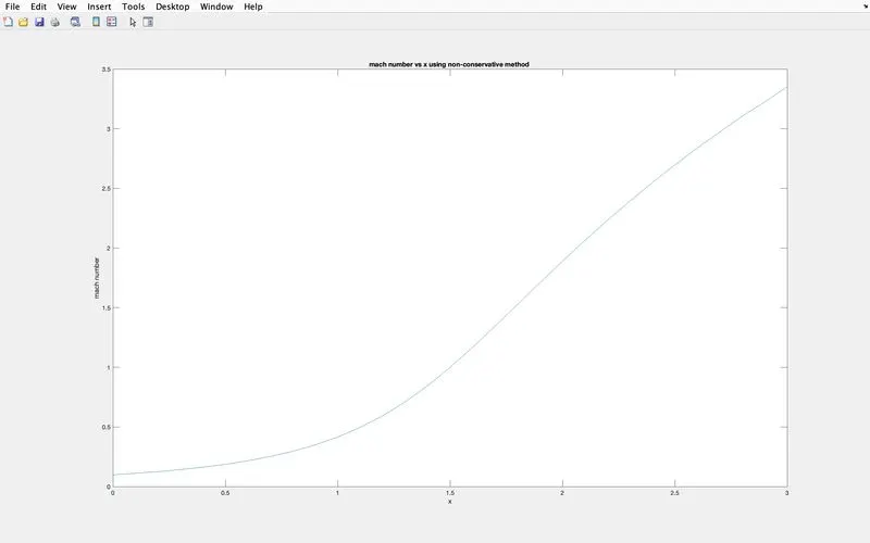
Here we can conclude that in the non-conservative form as x increases mach number also increases which is understandable as the velocity also increases and the nozzle is a subsonic-supersonic nozzle. Along the length the mach number varies from less than 1 to greater than 1.
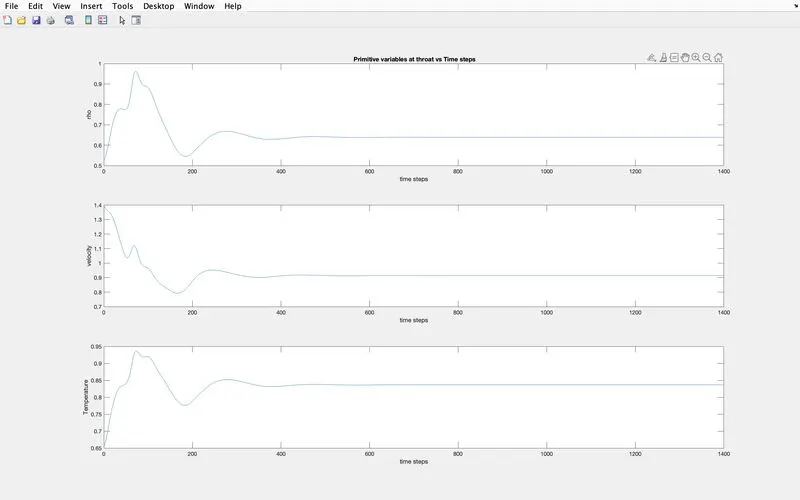
INFERENCE
Here as the time step increases the value of primitive variables rho_throat,t0_throat and v_throat becomes stable.
Program of Non-Conservative 1D nozzle flow
function m_dot_con = conv_func()
%inputs
nx = 31;
x = linspace(0,3,nx);
dx = x(2)-x(1);
gamma = 1.4;
c = 0.5
%time steps
nt = 1400;


%initial conditions
for i =1:nx
    if(x(i)>=0) && (x(i)<=0.5)
        rho(i) = 1;
        t0(i) = 1;

    elseif(x(i)>=0.5) && (x(i)<=1.5)
        rho(i) = 1-0.366*(x(i)-0.5);
        t0(i) = 1-0.167*(x(i)-0.5);
    elseif(x(i)>=1.5) && (x(i)<=3)
        rho(i) = 0.634-0.3879*(x(i)-1.5);
        t0(i) = 0.833-0.3507*(x(i)-1.5);
    end
end

a = 1+2.2*(x-1.5).^2;
v = 0.59./(rho.*a);
sound = sqrt(t0);
%solution vector
u1 = rho.*a;
u2 = rho.*a.*v;
u3 = rho.*((t0./(gamma-1))+(gamma/2)*v.^2).*a;

for k = 1:nt
    dt1 = (c*dx)./(sound+v);
    dt = min(dt1);
    u1old = u1;
    u2old = u2;
    u3old = u3;

    f1 = u2;
    f2 = (u2.^2./u1)+((gamma-1)/gamma)*(u3-(gamma/2)*(u2.^2)./u1);
    f3 = gamma*((u2.*u3)./u1)-gamma*(gamma-1)/2*(u2.^3./u1.^2);


    %predictor method
    for i = 2:nx-1
        %continuity equation
        du1_dt_p(i) = -(f1(i+1)-f1(i))/dx;
        %momentum equation
        du2_dt_p(i) = -((f2(i+1)-f2(i))/dx)+(1/gamma)*rho(i)*t0(i)*((a(i+1)-a(i))/dx);
        %energy equation
        du3_dt_p(i) = -(f3(i+1)-f3(i))/dx;

        %solution update
        u1(i) = u1old(i)+du1_dt_p(i)*dt;
        u2(i) = u2old(i)+du2_dt_p(i)*dt;
        u3(i) = u3old(i)+du3_dt_p(i)*dt;


    end

        rho = u1./a;
        v =u2./u1;
        t0 = (gamma-1)*((u3./u1)-(gamma/2)*v.^2);
        p = rho.*t0;
      %flux values update
        f1 = u2;
        f2 = (u2.^2./u1)+((gamma-1)/gamma)*(u3-(gamma/2)*(u2.^2)./u1);
        f3 = gamma*((u2.*u3)./u1)-gamma*(gamma-1)/2*(u2.^3./u1.^2);

    %corrector step
    for i = 2:nx-1
        %continuity equation
        du1_dt_c(i) = -(f1(i)-f1(i-1))/dx;
        %momentum equation
        du2_dt_c(i) = -((f2(i)-f2(i-1))/dx)+(1/gamma)*rho(i)*t0(i)*((a(i)-a(i-1))/dx);
        %energy equation
        du3_dt_c(i) = -(f3(i)-f3(i-1))/dx;


    end
    %average time update
    du1_dt_avg = 0.5*(du1_dt_c+du1_dt_p);
    du2_dt_avg = 0.5*(du2_dt_c+du2_dt_p);
    du3_dt_avg = 0.5*(du3_dt_c+du3_dt_p);

    %final solution update
    for i = 2:nx-1
        u1(i) = u1old(i)+(du1_dt_avg(i))*dt;
        u2(i) = u2old(i)+(du2_dt_avg(i))*dt;
        u3(i) = u3old(i)+(du3_dt_avg(i))*dt;
    end

    %initial conditions
    u1(1) = rho(1)*a(1);
    u2(1) = 2*u2(2)-u2(3);
    u3(1) = u1(1)*((t0(1)/(gamma-1))+(gamma/2)*v(1)^2);

    % boundary condtions
    u1(nx) = 2*u1(nx-1)-u1(nx-2);
    u2(nx) = 2*u2(nx-1)-u2(nx-2);
    u3(nx) = 2*u3(nx-1)-u3(nx-2);

    %primitive variables
    rho = u1./a;
    v =u2./u1;
    t0 = (gamma-1)*((u3./u1)-(gamma/2)*v.^2);
    p = rho.*t0;


    %plotting
    figure(5)
    subplot(3,1,1)
    plot(x,rho)
    xlabel('x')
    ylabel('rho')
    title('Primitive variables against x in the conservative form')

    subplot(3,1,2)
    plot(x,v)
    xlabel('x')
    ylabel('v')
    subplot(3,1,3)
    plot(x,t0)
    xlabel('x')
    ylabel('t0')

    pause(0.03)

    u1_throat(k) = u1(16);
    u2_throat(k) = u2(16);
    u3_throat(k) = u3(16);
    m_dot_con = rho.*a.*v;
    if (k==100)
        figure(6)
     plot(x,m_dot_con)
     hold on
    elseif (k==200)
         figure(6)
      plot(x,m_dot_con)
     elseif (k==500)
         figure(6)
      plot(x,m_dot_con)
     elseif (k==700)
         figure(6)
     plot(x,m_dot_con)
     xlabel('x')
     ylabel('m_dot_con')
     legend('k==100','k==200','k==500','k==700')
     title('Mass flow rate at varying time steps for conservative form')

    end

end
%mach number
m = v./sqrt(t0);
figure(7)
plot(x,m)
xlabel('x')
ylabel('mach number')
 title('mach number vs x using conservative method ')
%plotting
figure(8)
subplot(3,1,1)
plot(u1_throat)
xlabel('number of time steps')
ylabel('u1_throat')
title(' Solution variables at throat vs Time steps')
subplot(3,1,2)
plot(u2_throat)
xlabel('number of time steps')
ylabel('u2_throat')
subplot(3,1,3)
plot(u3_throat)
xlabel('number of time steps')
ylabel('u3_throat')


end
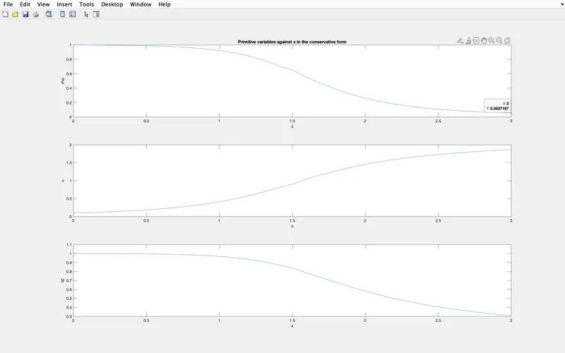
INFERENCE
In the above plot we understand that as the value of x increases velocity v increases i.e as the fluid flows through the nozzle the velocity of the fluid inside the nozzle increases and density and temperature decreases as x increases.
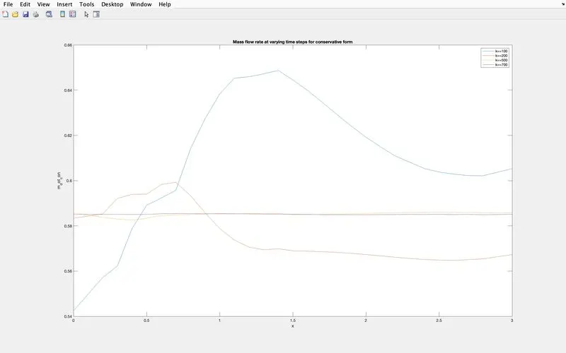
INFERENCE
In the above plot we have shown mass flow rate at different time steps(k) as k increases we can see that the plot gets linear and becomes similar to each other. This shows that the value of mass flow rate at higher time steps are stable, making the program reliable.
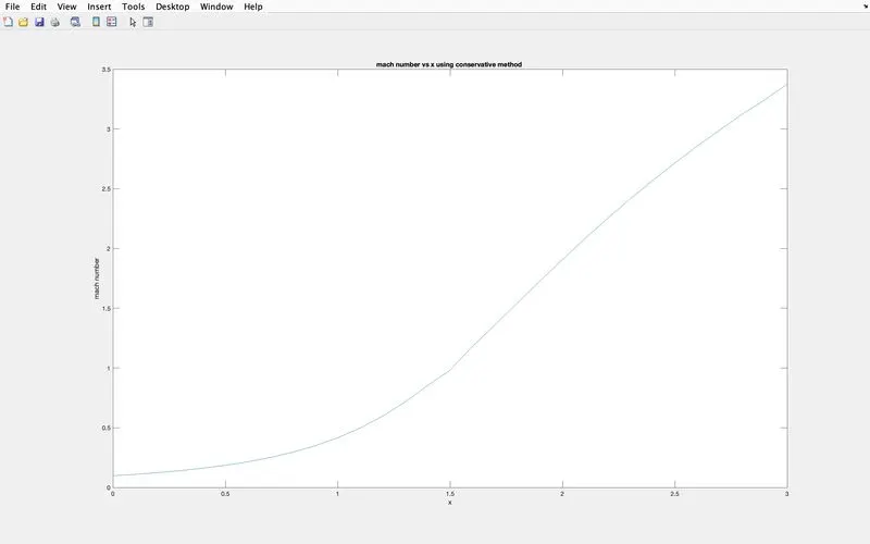
INFERENCE
Here we can conclude that in the conservative form as x increases mach number also increases which is understandable as the velocity also increases and the nozzle is a subsonic-supersonic nozzle. Along the length the mach number varies from less than 1 to greater than 1.
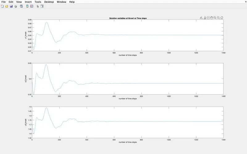
INFERENCE
Here as the time step increases the value of solution variables u1_throat, u2_throat and u3_throat becomes stable. We can see that from time step =500 onwards the plot is a horizontal straight line for all the three plots.
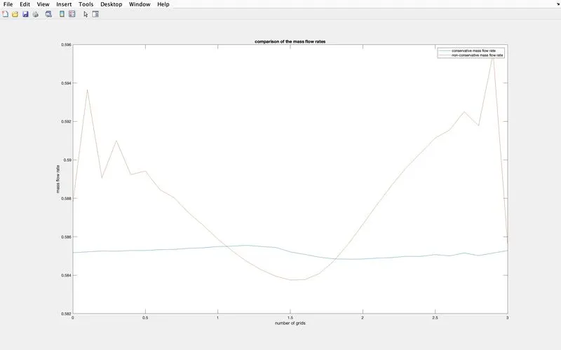
INFERENCE
Here in the above plot eventhough the final solution of both the forms are almost similar, the Non Conservative form oscillates much when compared to Conservative form. The latter also gives almost stable solution along the length. By this we can conclude that Conservative form attains stability in lesser number of iterations with earliest time.
RESULT
After completing the progarm we can conclude that Conservative form attains stability in lesser number of iterations with earliest time. Thus Conservative form is more stable than the Non-conservative form.
Grid Independence Test
This test is done to check whether the values of density, temperature, velocity and mach number at different number of grid points are close to each other or in other words the values should not be having a big difference between them. Here we calculated the density, velocity, temperature and mach number of both conservative and non-conservative method at nx = 31 and nx =61 and the following values are noted.
| Conservative Method | Non Conservative Method |
| nx = 31 | nx = 61 | nx = 31 | nx = 61 | |
| Density | 0.9971 | 0.9988 | 0.9970 | 0.9988 |
| Temperature | 0.9989 | 0.9998 | 0.9988 | 0.9998 |
| Pressure | 0.9960 | 0.9983 | 0.9428 | 0.9461 |
| Velocity | 0.1244 | 0.1098 | 0.1252 | 0.1099 |
| Mach number | 0.1245 | 0.1099 | 0.1253 | 0.1099 |
It is clear from the above table that the values are almost same along all the Primitive Variables for both the forms even when the Grid points(nx) is changed from 31 to 61 showcasing that it doesn't get affected by the increase of Grid points.
CONCLUSION
The program to Simulate the isentropic flow through a Quasi 1D subsonic nozzle by deriving both the conservation and non-conservation forms of the governing equations and solve them by implementing the MacCormack's technique using MATLAB is successfully completed and the required values and plots are noted down