Week 7 - Simulation of a 1D Super-sonic nozzle flow simulation using Macormack Method

• AIM:

The main aim of the project is to write the code to simulate the Conservative and Non-conservative form of Quasi one-dimenstional Nozzle flows using Macormack method and compare with the exact results.

• OBJECTIVE:

INTRODUCTION TO SUBSONIC-SUPERSONIC ISENTROPIC FLOW:

We consider the steady,isentropic flow through a convergent-divergent nozzle as shown in the figure(reference: Computational Fluid Dynamics by JOHN D ANDERSON).The flow at the inlet to the nozzle comes from a reservoir where the pressure and temperature are denoted by `p_0` and `T_0`,respectively.The cross-sectional area of the reservoir is large(theoretically,A-->`infty`),and hence the velocity is very small(V-->0).Thus `p_0` and `T_0` are stagnation values,or total pressure and total temperature respectively.The flow expands isentropically to supersonic speeds at the nozzle exit,where the exit pressure,temperature,velocity and mach number are denoted by `p_e,T_e,V_e` and `M_e`,respectively.The flow is locally subsonic in the convergent section of the nozzle,sonic at the throat,and supersonic at the divergent section.The sonic flow at the throat means that the local velocity at this location is equal to the local speed of sound.We assume that at a given section,where the cross-sectional area is A ,the flow properties are uniform across that section.Hence,although the area of the nozzle changes as a function of the distance along the nozzle,x, and therfore in relaity the flow field is two dimensional,we make the assumption that the flow properties vary only with x,such flow is defined as quasi-one-dimensional flow.

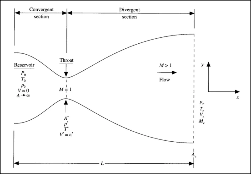
The governing continuity,momentum, and energy equations for quasi-one-dimensional,stady,isentropic flow can be expresses,respectively,as

Continuity: `rho_1V_1A_1=rho_2V_2A_2`

Momentum: `p_1A_1+rho_1V_1^2A_1+int_(A_1)^(A_2)pdA=p_2A_2+rho_2V_2^2A_2`

Energy: `h_1+(V_1^2)/2=h_2+(V_2^2)/2`

The above equations can be solved analytically for the flow through the nozzle.The mach number variation through the nozzle is governed exclusively by the area ratio `A/A^ast` through the relation

`(A/A^ast)^2=1/M^2[2/(gamma+1)(1+(gamma-1)/2)M^2]^((gamma+1)/(gamma-1)`

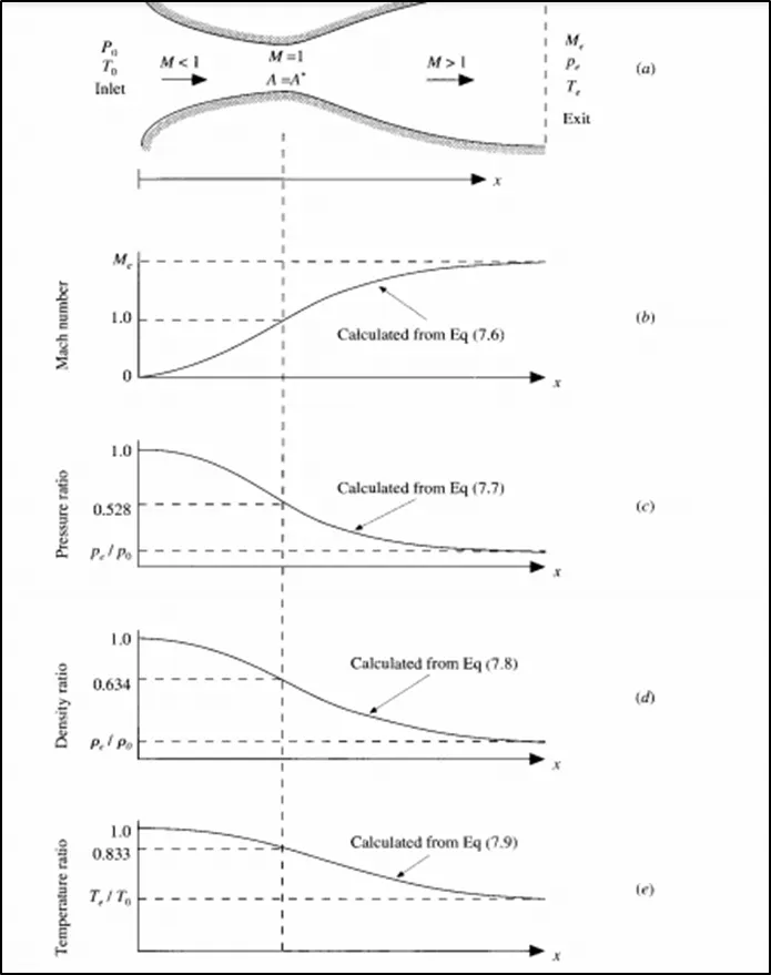
where `gamma`= ratio of specific heats.For air standard conditions,`gamma =1.4`.For a nozzle where A is specified as a function of x,hence `A/A^ast`is known as function of x.The variation of pressure ,density and temperature as a function of Mach number is given respectively by,

`p/p_0=(1+(gamma-1)/2M^2)^(-gamma/(gamma-1))`

`rho/rho_0=(1+(gamma-1)/2M^2)^(-1/(gamma-1))`

`T/T_0=(1+(gamma-1)/2M^2)^-1`

these variation are shown in the figure(reference: Computational Fluid Dynamics by JOHN D ANDERSON),

• MACCORMACK'S TECHNIQUE:

Maccormack technique is an explicit finite-difference technique which is second-order-accurate in both space and time.

let us consider the density at grid point(i,j) at time `t+Deltat`.In MacCormack's method,this is obtained from

`rho_(i,j)^(t+Deltat)=rho_(i,j)^t+((delrho)/(delt))_(avg)Deltat` where `((delrho)/(delt))_(avg)` is a representative mean value of `(delrho)/(delt)` between t and `t+Deltat`

similar relations are written for the other flow field variables

`u_(i,j)^(t+Deltat)=u_(i,j)^t+((delu)/(delt))_(avg)Deltat`

`T_(i,j)^(t+Deltat)=T_(i,j)^t+((delT)/(delt))_(avg)Deltat`

Let us illustrate the calculation of density

Predictor step:

Continuity equation i `(delrho)/(delt)=-(rho(delu)/(delx)+u(delrho)/(delx)+rho(delv)/(dely)+v(delrho)/(dely))`

relpace the spatial derivatives on right hand side with forward differences.

`((delrho)/(delt))_(i,j)^t=-(rho_(i,j)^t(u_(i+1,j)^t-u_(i,j)^t)/(Deltax)+u_(i,j)^t(rho_(i+1,j)^t-rho_(i,j)^t)/(Deltax)+rho_(i,j)^t(v_(i+1,j)^t-v_(i,j)^t)/(Deltay)+v_(i,j)^t(rho_(i+1,j)^t-rho_(i,j)^t)/(Deltay))`

All flow variables at time t are known values,now obtain a predicted value of density

`rho_(i,j)^(t+Deltat)=rho_(i,j)^t+((delrho)/(delt))_(i,j)^tDeltat`

In similar fashion,predicted values of u and T can be obtained

`u_(i,j)^(t+Deltat)=u_(i,j)^t+((delu)/(delt))_(i,j)^tDeltat`

`v_(i,j)^(t+Deltat)=v_(i,j)^t+((delv)/(delt))_(i,j)^tDeltat`

`T_(i,j)^(t+Deltat)=T_(i,j)^t+((delT)/(delt))_(i,j)^tDeltat`

The value `rho_(i,j)^(t+Deltat)` is only a predicted value of density;it is only first-order-accurate.

Corrector step:

In the corrector step,we first obtain a predicted value of the time derivative at time `t+Deltat`,by substituting the predicted values of `rho,u,v` into the right hand side of the continuity equation,replacing the spatial derivative with reward differences.

`((delrho)/(delt))_(i,j)^(t+Deltat)=-(rho_(i,j)^(t+Deltat)(u_(i,j)^(t+Deltat)-u_(i-1,j)^(t+Deltat))/(Deltax)+u_(i,j)^(t+Deltat)(rho_(i,j)^(t+Deltat)-rho_(i-1,j)^(t+Deltat))/(Deltax)+rho_(i,j)^(t+Deltat)(v_(i,j)^(t+Deltat)-v_(i,j-1)^(t+Deltat))/(Deltay)+v_(i,j)^(t+Deltat)(rho_(i,j)^(t+Deltat)-rho_(i,j-1)^(t+Deltat))/(Deltay))`

The average value of the time derivative of density can be obtained from the equation

`((delrho)/(delt))_(avg)=1/2[((delrho)/(delt))_(i,j)^t+((delrho)/(delt))_(i,j)^(t+Deltat)]`

This allows us to obtain the final correcetd value of density at time `t+Deltat`

`rho_(i,j)^(t+Deltat)=rho_(i,j)^t+((delrho)/(delt))_(avg)Deltat`

This sequence is repeated at all grid points to obtain the density throughout the flow field at time `t+Deltat`.

To calculate u,v and T at time `t+Deltat`,the same technique is used.

CFD SOLUTION OF SUBSONIC-SUPERSONIC ISENTROPIC NOZZLE FLOW:

Generally,for nozzle flows,the flow field variables are frequently expressend interms of nondimensional variables,where flow variables are referenced to their reservoir values

NON-CONSERVATIVE FORM OF GOVERNING EQUATION:

Continuity: `(delrho')/(delt')=-rho'(delV')/(delx')-rho'V'((del(lnA'))/(delx'))-V'(delrho')/(delx')`

Momentum: `(delV')/(delt')=-V'(delV')/(delx')-1/gamma((delT')/(delx')+(T')/(rho')(delrho')/(delx'))`

Energy: `(delT')/(delt')=-V'(delT')/(delx')-(gamma-1)T'[(delV')/(delx')+V'((del(lnA')))/(delx')]`

where `T'=T/T_0 and rho'=rho/rho_0` and `x'=x/L`

`a_0=sqrt(gammaRT_0)` and also we define dimentionless velocity as `V'=V/a_0`

Grid point distribution along the nozzle is given in the figure (reference: Computational Fluid Dynamics by JOHN D ANDERSON)

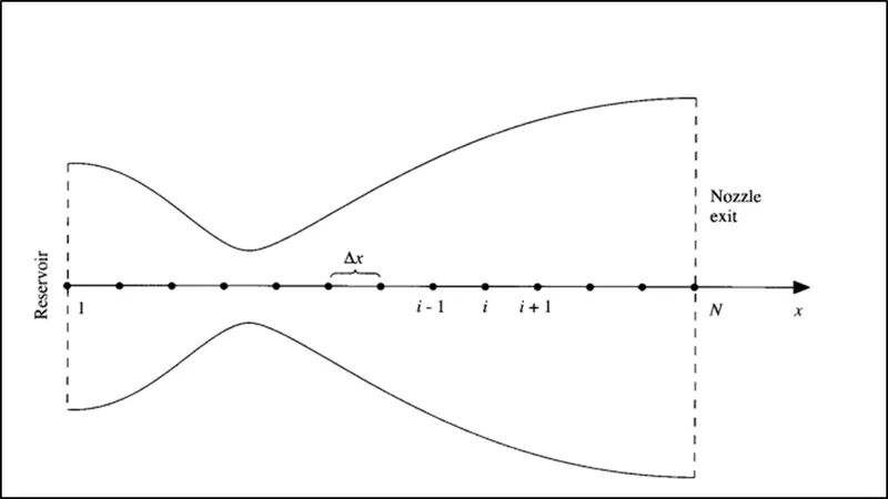
MacCormack technique is used to solve the above governing equation as explained earlier and obtain the correct value of the density,velocity and temperature of the flow.

CALCULATION OF TIMESTEP:

Calculate `(Deltat)_i^t` at all the grid points,i=1 to i=n,and then choose the minimum value of `Deltat`.That is,

`Deltat=min(Deltat_1^t,Deltat_2^t,Deltat_3^t,.....,Deltat_n^t)`

BOUNDARY CONDITON:

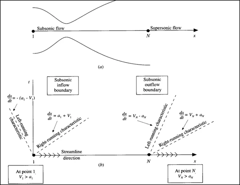
In the above figure Point 1 is essentially in the reservoir;it represents an inflow boundary,with flow coming from the reservoir and entering the nozzle.Point N is an outflow boundary,with flow leaving the nozzle at the nozzle exit.

We know that unsteady,inviscid flow is governed by hyperbolic equations,and therefore for one-dimensional unsteady flow their exist two real characteristic lines.At point1,the local flow velocity is subsonic,V1

SUBSONIC INFLOW BOUNDARY(Point 1):

Here,we must allow one variable to float;we choose the velocity V1,because on a physical basis we know the mass flow through the nozzle must be allowed to adjust to the proper steady state,we use linear extrapolation from point 2 and 3 to calculate V1 ,

slope=`(V_3-V_2)/(Deltax)`

using slope we find V1 by linear extrapolation we get

`V_1=V_2-(V_3-V_2)/(Deltax)Deltax`

`V_1=2V_2-V_3`

SUPERSONIC OUTFLOW BOUNDARY(Point N):

Here,we must allow all flow-field variables to float.We againg choose to use linear extrapolation based on the flow field values at the internal points.

`V_N=2V_(N-1)-V_(N-2)`

`rho_N=2rho_(N-1)-rho_(N-2)`

`T_N=2T_(N-1)-T_(N-2)`

NOZZLE SHAPE AND INITIAL CONDITION:

We choose a parabolic area distribution given by,

`A=1+2.2(x-1.5)^2`

We know that `rho and T` decreases and V increases as the flow expands through the nozzle ,we choose initial condition that qualitatively behave in same fashion,we assume following values at time t=0

`rho=1-0.3146x`

`T=1-0.2314x`

`V=(0.1+1.09x)T^(1/2)`

• CODING FOR NON-CONSERVATIVE FORM:

% 1D supersonic nozzel flow (Non-Conservative form)

clear all
close all
clc

%Domain length
L=3;
n=31;
x=linspace(0,L,n);
dx = x(2)-x(1);
gamma = 1.4;

%Initial condition at t=0

rho_initial = 1-(0.3146*x);
T_initial = 1-(0.2314*x);
u_initial = (0.1+1.09*x).*T_initial.^0.5;

%Nozzle shape
A = 1+2.2*(x-1.5).^2;

%Grid point for throat of nozzle at x =1.5
th = find(A==1);

%Field variables
rho = rho_initial;
T= T_initial;
u=u_initial;

%Calculation of time step dt

CFL = 0.5;
for z = 1:n
    dt_ini(z)=CFL*((dx)/((T_initial(z)^0.5)+u_initial(z)));
    
end
dt = min(dt_ini);

%Number of iteration
n_iter = 1400;
t_sim = (n_iter-1)*dt;
t = 0:dt:t_sim ;


%Maccormack method
for k=1:length(t)
        rho_old = rho;
        T_old = T;
        u_old = u;
    
    for i=2:(n-1)
        %Defining spacial derivatives
        du_dx = (u(i+1)-u(i))/dx;
        dlnA_dx=(log(A(i+1))-log(A(i)))/dx;
        drho_dx = (rho(i+1)-rho(i))/dx;
        dT_dx = (T(i+1)-T(i))/dx;
        
        %Predictor step
        
        %Continuity equation
        drho_dt_p(i)=-rho(i)*du_dx-rho(i)*u(i)*dlnA_dx-u(i)*drho_dx;
        
        %Momentum Equation
        du_dt_p(i)=-u(i)*du_dx-(1/gamma)*(dT_dx+(T(i)/rho(i))*drho_dx);
        
        %Energy Equation
        dT_dt_p(i)=-u(i)*dT_dx-((gamma-1)*T(i)*(du_dx+(u(i)*dlnA_dx)));
        
        %Step update
        rho(i)=rho_old(i)+(drho_dt_p(i)*dt);
        u(i)=u_old(i)+(du_dt_p(i)*dt);
        T(i)=T_old(i)+(dT_dt_p(i)*dt);
        
        
    end
    for i=2:(n-1)
        %Defining spacial derivatives
        du_dx = (u(i)-u(i-1))/dx;
        dlnA_dx=(log(A(i))-log(A(i-1)))/dx;
        drho_dx = (rho(i)-rho(i-1))/dx;
        dT_dx = (T(i)-T(i-1))/dx;
        
        %Corrector step
        
        %Continuity equation
        drho_dt_c(i)=-rho(i)*du_dx-rho(i)*u(i)*dlnA_dx-u(i)*drho_dx;
        
        %Momentum Equation
        du_dt_c(i)=-u(i)*du_dx-(1/gamma)*(dT_dx+(T(i)/rho(i))*drho_dx);
        
        %Energy Equation
        dT_dt_c(i)=-u(i)*dT_dx-((gamma-1)*T(i)*(du_dx+(u(i)*dlnA_dx)));
  
       
    end
    %Computing average Time derivative
     for j =2:n-1
        drho_dt_avg(j)=0.5*( drho_dt_p(j)+drho_dt_c(j));
        du_dt_avg(j)=0.5*( du_dt_p(j)+du_dt_c(j));
        dT_dt_avg(j)=0.5*( dT_dt_p(j)+ dT_dt_c(j));
    
    %Final update
   
       rho(j)=rho_old(j)+ drho_dt_avg(j)*dt;
       u(j)=u_old(j)+du_dt_avg(j)*dt;
       T(j)=T_old(j)+dT_dt_avg(j)*dt;
    end
    
    %Boundary Conditions
    %Inflow Boundary
    u(1)=(2*u(2))-u(3);
    
    %Outflow Boundary
    u(n)=(2*u(n-1))-u(n-2);
    rho(n)=(2*rho(n-1))-rho(n-2);
    T(n)=(2*T(n-1))-T(n-2);
    
    %Pressure ratio
    p=rho.*T;
    
    %Mach number
    M=u./(T.^0.5);
    
    %Mass Flow Rate
    mass=rho.*u.*A;
    
    %Field Variable at Throat section
    rho_throat(k)=rho(th);
    T_throat(k)=T(th);
    M_throat(k)=M(th);
    p_throat(k)=p(th);
    
   
    
    
    %Plot for mass conservation
   mass_conservation(x,k,mass)
    
end

    %Plots for Timewise variation of rho,T,P,M at the nozzle throat
   plot_throat_1(rho_throat,T_throat,M_throat,p_throat); 
   %Qualitative aspects of quasi-one-dimensional nozzle flow
   steady_state(x,M,T,p,rho)
   
  
   

CODE FOR PLOTS:

Non-dimensional mass flow as a function of distance through the nozzle

function[]=mass_conservation(x,k,mass)


figure(7)

hold on
if(k==1)
    plot(x,mass,'--')
    
elseif(k==51)
    plot(x,mass,'g')
elseif(k==101)
    plot(x,mass,'r')
elseif(k==151)
    plot(x,mass,'c')
elseif(k==201)
    plot(x,mass,'y')
elseif(k==701)
    plot(x,mass,'black')
    legend('0dt','50dt','100dt','150dt','200dt','700dt')
    xlabel('Non-dimentional distance through nozzle')
    ylabel('Non-dimentional mass flow rate at different instances')
    grid on
    
    
end

Time-wise variation of the density,temperature,pressure and mach number at the nozzle throat

function[]= plot_throat_1(rho_throat,T_throat,M_throat,p_throat)
%Exact analytical solution at throat section
rho_exact = 0.634*ones(1,1400);
T_exact = 0.833*ones(1,1400);
M_exact=1*ones(1,1400);
p_exact=0.528*ones(1,1400);

%Plots for convergence
figure(1)
plot(rho_throat)
hold on
plot(rho_exact)
axis([0 1400 0.5 1])
xlabel('Number of timestep')
ylabel('Density')
legend('Numerical solution','Exact solution')
title('Density at throat section')


figure(2)
plot(T_throat)
hold on
plot(T_exact)
axis([0 1400 0.65 1])
xlabel('Number of timestep')
ylabel('Temperature')
legend('Numerical solution','Exact solution')
title('Temperature at throat section')

figure(3)
plot(M_throat)
hold on
plot(M_exact)
axis([0 1400 0.8 1.8])
xlabel('Number of timestep')
ylabel('Mach Number')
legend('Numerical solution','Exact solution')
title('Mach Number at throat section')

figure(4)
plot(p_throat)
hold on
plot(p_exact)
axis([0 1400 0 1])
xlabel('Number of timestep')
ylabel('Pressure Ratio')
legend('Numerical solution','Exact solution')
title('Pressure ratio at throat section')
end

Variation of density,temperature,pressure ratio and mach number with respect to x:

function[]=steady_state(x,M,T,p,rho)

figure(5)
subplot(4,1,1)
plot(x,M)
axis([0 3 0 4])
xlabel('x')
ylabel('Mach Number')
legend('Mach Number')
grid minor
subplot(4,1,2)
plot(x,T)
axis([0 3 0 1.5])
xlabel('x')
ylabel('Temperature')
legend('Temperature')
grid minor
subplot(4,1,3)
plot(x,p)
axis([0 3 0 1.5])
xlabel('x')
ylabel('pressure')
legend('pressure')
grid minor
subplot(4,1,4)
plot(x,rho)
axis([0 3 0 1])
xlabel('x')
ylabel('Density')
legend('Density')
grid minor
end

• EXPLANATION:

1. Initialize the code by providing the domain length,number of nodes,gamma value.
2. Provide the initial conditions of density,temperature,velocity at time t=0.
3. Calculate the time step using CFL of 0.5.
4. Provide the nozzle shape value as area varies with x
5. Find the node value at throat and store in the variable called th.
6. Initalize the maccormack method for the length of t and find the predicited values and then update the values and use those values in corrector step to find the correct values of the variables.
7. Apply the boundary condition at inflow and outflow.
8. Plot for timewise variation and steady state variation of density ,temperature,pressure ratio,Mach number and compare with the exact values.

• OUTPUT:

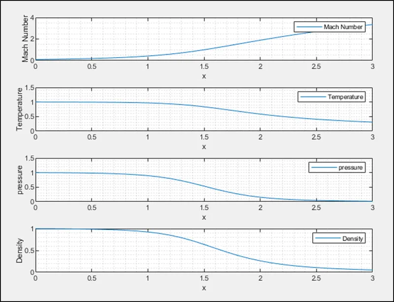
The above plot shows the variation of Mach number,pressure ratio,Density ratio and Temperature ratio with respect to the x,and it varies as expected the temperature ,pressure and density decreases as flow expands and Mach number increases and variation are similar to the variation shown in the John D Anderson book.

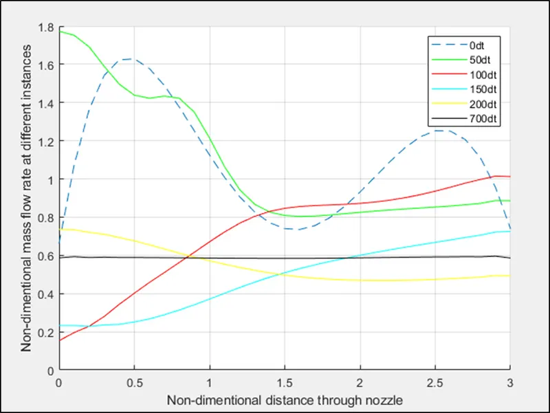
In this plot the non-dimensional mass flow `rhoAV`is plotted as a function of Non-dimentional distance through nozzle.Six different curves are shown,each for a different time during the course of the time-marching procedure.The dashed curve is simply the product of the assumed initial condition `rhoAV`,and hence labelled as `0Deltat`.After 50 time step,the mass flow distribution through the nozzle has changed considerably;this given by the curve labeled `50Deltat`.After 100time step,the mass flow distribution has changed radically;the mass flow variation is simply flopping around inside the nozzle due to the transient variation of the flow-field variables.Howevere,after 200 time steps,the mass flow distribution is beginning to settle down,and after 700 timesteps,the mass flow distribution is a straight,horizontal line across the graph.This says that the mass flow has converged to a constant,steady-state value throughout the nozzle.

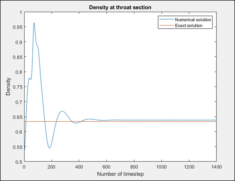
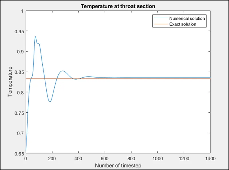
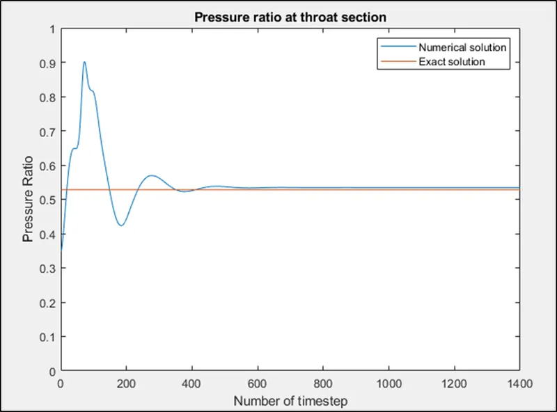
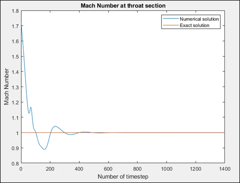
In the above four plots we can observe the time-wise variation of density,temperature,Pressure and mach number at the nozzle throat v/s the number of time steps.The red line in the plot represents exact,analytical values as obtained.We can observe from the plots that the numerical time-marching procedure converges to the proper theoretical steady-state answer.

• GRID INDEPENDENCE TEST:

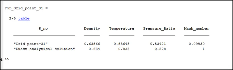
For n=31

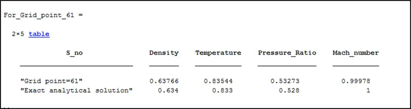
For n=61

COMPARISION:

	`rho^ast/rho_0`	`T^ast/T_0`	`p^ast/p_0`	M
31 points	0.638	0.836	0.534	0.999
61 points	0.637	0.835	0.532	0.999
Exact analytical solution	0.634	0.833	0.528	1.000

Table compares the steady-state results of density,temperature,pressure and mach number at the throat for both the cases using 31 and 61 grid points and also compares with the exact analytical solution ,we observe that by doubling the number of grid points numerical soution improves marginally,so we can conclude that our original calculation using 31 grid points is essentially grid-independent.

CONSERVATIVE FORM OF GOVERNING EQUATION:

CONTINUITY: `(del(rho'A'))/(delt')+(del(rho'A'V'))/(delx')=0`

MOMENTUM: `(del(rho'A'V'))/(delt')+(del(rho'A'V'^2+(1/gamma)p'A'))/(delx')=1/gammap'(delA')/(delx')`

ENERGY: `(del(rho'((T')/(gamma-1)+gamma/2V'^2)A'))/(delt')``+(del[rho'((T')/(gamma-1)+gamma/2V'^2)V'A'+p'A'V'])/(delx')=0`

The equations for quasi-one-dimensional flow can be expressed in a generic form.Let us define the elements of the solution vector U,the flux vector F,and the source term J as follows

`U_1=rho'A'`

`U_2=rho'A'V'`

`U_3=rho'((T')/(gamma-1)+gamma/2V'^2)A'`

`F_1=rho'A'V'`

`F_2=rho'A'V'^2+1/gammap'A'`

`F_3=rho'((T')/(gamma-1)+gamma/2V'^2)V'A'+p'A'V'`

`J_2=1/gammap'(delA')/(delx')`

with these the governing equations can be written as,

`(delU_1)/(delt')=-(delF_1)/(delx')`

`(delU_2)/(delt')=-(delF_2)/(delx')+J_2`

`(delU_3)/(delt')=-(delF_3)/(delx')`

To obtain primitive variables we should decode the elements U1,U2 and U3 as follows,

`rho'=U_1/(A')` `V'=U_2/U_1` `T'=(gamma-1)(U_3/U_2-gamma/2V'^2)`

PURE FORM OF THE FLUX TERMS:

`F_1=U_2`

`F_2=U_2^2/U_1+(gamma-1)/gamma(U_3-gamma/2U_2^2/U_1)`

`F_3=gamma(U_2U_3)/U_1-(gamma(gamma-1))/2U_2^3/U_1^2`

• BOUNDARY CONDITIONS:

The boundary conditions for subsonic-supersonic isentropic flow solution using the conservative form of the governing equation are theoritacally same as discussed earlier.In this senario,we hold `rho' and T'`fixed at the inflow boundary,both equal to 1,and allow`V'` to float

INFLOW BOUNDARY CONDITIONS:

`U_1=rho'A'`

`U_2(1)=2U_2(2)-U_2(3)`

`U_3=U_1((T')/(gamma-1)+gamma/2V'^2)`

OUTFLOW BOUNDARY CONDITIONS:

`U_1(N)=2U_1(N-1)-U_1(N-2)`

`U_2(N)=2U_2(N-1)-U_2(N-2)`

`U_3(N)=2U_3(N-1)-U_3(N-2)`

• INITIAL CONDITIONS:

For this calculations the same nozzle shape is used.The initial conditions for U1,U2,U3 were synthesized by assuming the following variations of `rho' and T'`

`rho'=1.0 and T'=1.0` for `0lex'le0.5`

`rho'=1.0-0.366(x'-0.5)and T'=1.0-0.167(x'-0.5)` for `0.5lex'le1.5`

`rho'=0.634-0.3879(x'-1.5) and T'=0.833-0.3507(x'-1.5)` for `1.5lex'le3.5`

`V'=U_2/(rho'A')=0.59/(rho'A')`

• CALCULATION OF TIME STEP:

The governing equations for unsteady,quasi-one-dimensional flow in conservation form are hyperbolic partial differential equations,just as are the governing equations in non-conservation form which is used earlier,therfore the calculation of time step is same as explained earlier.

• CODING FOR CONSERVATION FORM OF GOVERNING EQUATION:

% 1D supersonic nozzel flow (Conservative form)

clear all
close all
clc

%Domain length
L=3;
n=31;
x=linspace(0,L,n);
dx = x(2)-x(1);
gamma = 1.4;

%Initial conditiona
for i=1:n
   if(x(i)<=0.5)
       rho_initial(i)=1;
       T_initial(i)=1;
   elseif(x(i)>0.5)&&(x(i)<=1.5)
       rho_initial(i)=1-(0.366*(x(i)-0.5));
        T_initial(i)=1-(0.167*(x(i)-0.5));
   else
       rho_initial(i)=0.634-(0.3879*(x(i)-1.5));
       T_initial(i)=0.833-(0.3507*(x(i)-1.5));
   end
end
 
%Nozzle shape
A = 1+2.2*(x-1.5).^2;
%Initial velocity 
 u_initial=0.59./(rho_initial.*A);
 
%Grid point for throat of nozzle at x =1.5
th = find(A==1);

%Field variables
rho = rho_initial;
T= T_initial;
u=u_initial;

%Calculation of time step dt

CFL = 0.5;
for z = 1:n
    dt_ini(z)=CFL*((dx)/((T_initial(z)^0.5)+u_initial(z)));
    
end
dt = min(dt_ini);

%Number of iteration
n_iter = 1400;
t_sim = (n_iter-1)*dt;
t = 0:dt:t_sim ;

%Solution vector u
U1_initial=rho_initial.*A;
U2_initial=rho_initial.*A.*u_initial;
U3_initial=rho_initial.*A.*((T_initial/(gamma-1)+(gamma/2)*(u_initial.^2)));

U1=U1_initial;
U2=U2_initial;
U3=U3_initial;

%Maccormack method
for j=1:length(t)
    U1_old=U1;
    U2_old=U2;
    U3_old=U3;
    
    %Pure form of flux terms for predictor step
    F1=U2;
    F2=((U2.^2)./U1)+(((gamma-1)/gamma)*(U3-((gamma/2)*((U2.^2)./U1))));
    F3=gamma*((U2.*U3)./U1)-((gamma*((gamma-1))/2)*((U2.^3)./U1.^2));
    
    for k=2:(n-1)
        dA_dx=((A(k+1))-(A(k)))/dx;
        %source term
         J2=(1/gamma)*rho(k)*T(k)* dA_dx;
        
        %Predictor step
        
        %Continutiy equation
        dU1_dt_p(k)=-(F1(k+1)-F1(k))/dx;
        %Momentum equation
        dU2_dt_p(k)=-((F2(k+1)-F2(k))/dx)+J2;
        %Energy equation
        dU3_dt_p(k)=-(F3(k+1)-F3(k))/dx;
        
        %Step update
        U1(k)=U1_old(k)+(dU1_dt_p(k)*dt);
        U2(k)=U2_old(k)+(dU2_dt_p(k)*dt);
        U3(k)=U3_old(k)+(dU3_dt_p(k)*dt);
        
        
    end
     
    
    %Primitive variables
    
    rho=U1./A;
    u=U2./U1;
    T=(gamma-1)*((U3./U1)-(gamma/2)*(u.^2));
  
    
     %Pure form of flux terms for corrector step
    F1=U2;
    F2=((U2.^2)./U1)+(((gamma-1)/gamma)*(U3-((gamma/2)*((U2.^2)./U1))));
    F3=gamma*((U2.*U3)./U1)-((gamma*((gamma-1))/2)*((U2.^3)./U1.^2));
    
    for p=2:(n-1)
        dA_dx=((A(p))-(A(p-1)))/dx;
        %source term
        J2=(1/gamma)*rho(p)*T(p)* dA_dx;
        
        %corrector step
        
        %Continutiy equation
        dU1_dt_c(p)=-(F1(p)-F1(p-1))/dx;
        %Momentum equation
        dU2_dt_c(p)=-((F2(p)-F2(p-1))/dx)+J2;
        %Energy equation
        dU3_dt_c(p)=-(F3(p)-F3(p-1))/dx;
    end
    %Computing average Time derivative
       dU1_dt_avg=0.5*((dU1_dt_p+dU1_dt_c));
       dU2_dt_avg=0.5*((dU2_dt_p+dU2_dt_c));
       dU3_dt_avg=0.5*((dU3_dt_p+dU3_dt_c));
       
       
     for m =2:n-1 
          %Final update
         U1(m)=U1_old(m)+dU1_dt_avg(m)*dt;
         U2(m)=U2_old(m)+dU2_dt_avg(m)*dt;
         U3(m)=U3_old(m)+dU3_dt_avg(m)*dt;
     end
     
     %Boundary condition
     
     %Inflow condition
     U1(1)=rho(1)*A(1);
     U2(1)=2*U2(2)-U2(3);
     U3(1)=U1(1)*(((T(1))/(gamma-1))+(gamma/2)*u(1)^2);
     
     %Outflow condition
     U1(n)=2*U1(n-1)-U1(n-2);
     U2(n)=2*U2(n-1)-U2(n-2);
     U3(n)=2*U3(n-1)-U3(n-2);
     
     %Final values of primitive variables
     
    rho=U1./A;
    u=U2./U1;
    T=(gamma-1)*((U3./U1)-(gamma/2)*(u.^2));
    p=rho.*T;
    
    %Mach number
    M=u./(T.^0.5);
    
    %Mass Flow Rate
    mass=rho.*u.*A;
         
     %Field Variable at Throat section
    rho_throat(j)=rho(th);
    T_throat(j)=T(th);
    M_throat(j)=M(th);
    p_throat(j)=p(th); 
    
   

   %Plot for mass conservation
    mass_conservation_conservative(x,j,mass)

    
    
end
 %Plots for Timewise variation of rho,T,P,M at the nozzle throat
    plot_throat_1(rho_throat,T_throat,M_throat,p_throat); 
    %Qualitative aspexts of quasi-one-dimensional nozzle flow
    steady_state(x,M,T,p,rho)
    

    

CODE FOR PLOTS:

Non-dimensional mass flow as a function of distance through the nozzle

function[]=mass_conservation(x,k,mass)


figure(7)

hold on
if(k==1)
    plot(x,mass,'--')
    
elseif(k==51)
    plot(x,mass,'g')
elseif(k==101)
    plot(x,mass,'r')
elseif(k==151)
    plot(x,mass,'c')
elseif(k==201)
    plot(x,mass,'y')
elseif(k==701)
    plot(x,mass,'black')
    legend('0dt','50dt','100dt','150dt','200dt','700dt')
    xlabel('Non-dimentional distance through nozzle')
    ylabel('Non-dimentional mass flow rate at different instances')
    grid on
    
    
end

Time-wise variation of the density,temperature,pressure and mach number at the nozzle throat

function[]= plot_throat_1(rho_throat,T_throat,M_throat,p_throat)
%Exact analytical solution at throat section
rho_exact = 0.634*ones(1,1400);
T_exact = 0.833*ones(1,1400);
M_exact=1*ones(1,1400);
p_exact=0.528*ones(1,1400);

%Plots for convergence
figure(1)
plot(rho_throat)
hold on
plot(rho_exact)
axis([0 1400 0.5 1])
xlabel('Number of timestep')
ylabel('Density')
legend('Numerical solution','Exact solution')
title('Density at throat section')


figure(2)
plot(T_throat)
hold on
plot(T_exact)
axis([0 1400 0.65 1])
xlabel('Number of timestep')
ylabel('Temperature')
legend('Numerical solution','Exact solution')
title('Temperature at throat section')

figure(3)
plot(M_throat)
hold on
plot(M_exact)
axis([0 1400 0.8 1.8])
xlabel('Number of timestep')
ylabel('Mach Number')
legend('Numerical solution','Exact solution')
title('Mach Number at throat section')

figure(4)
plot(p_throat)
hold on
plot(p_exact)
axis([0 1400 0 1])
xlabel('Number of timestep')
ylabel('Pressure Ratio')
legend('Numerical solution','Exact solution')
title('Pressure ratio at throat section')
end

Variation of density,temperature,pressure ratio and mach number with respect to x:

function[]=steady_state(x,M,T,p,rho)

figure(5)
subplot(4,1,1)
plot(x,M)
axis([0 3 0 4])
xlabel('x')
ylabel('Mach Number')
legend('Mach Number')
grid minor
subplot(4,1,2)
plot(x,T)
axis([0 3 0 1.5])
xlabel('x')
ylabel('Temperature')
legend('Temperature')
grid minor
subplot(4,1,3)
plot(x,p)
axis([0 3 0 1.5])
xlabel('x')
ylabel('pressure')
legend('pressure')
grid minor
subplot(4,1,4)
plot(x,rho)
axis([0 3 0 1])
xlabel('x')
ylabel('Density')
legend('Density')
grid minor
end

• OUTPUT:

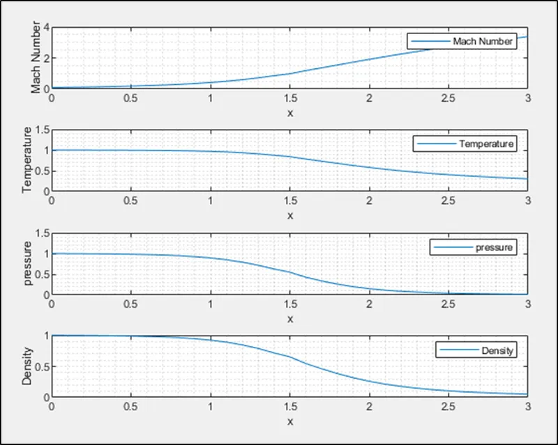
The above plot shows the variation of Mach number,pressure ratio,Density ratio and Temperature ratio with respect to the x,and it varies as expected the temperature ,pressure and density decreases as flow expands and Mach number increases and variation are similar to the variation shown in the John D Anderson book.

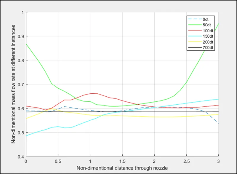
In this plot the non-dimensional mass flow `rhoAV`is plotted as a function of Non-dimentional distance through nozzle.Six different curves are shown,each for a different time during the course of the time-marching procedure.The dashed curve is simply the product of the assumed initial condition `rhoAV`,and hence labelled as `0Deltat`.After 50 time step,the mass flow distribution through the nozzle has changed considerably;this given by the curve labeled `50Deltat`.After 100time step,the mass flow distribution has changed radically;the mass flow variation is simply flopping around inside the nozzle due to the transient variation of the flow-field variables.Howevere,after 200 time steps,the mass flow distribution is beginning to settle down,and after 700 timesteps,the mass flow distribution is a straight,horizontal line across the graph.This says that the mass flow has converged to a constant,steady-state value throughout the nozzle.

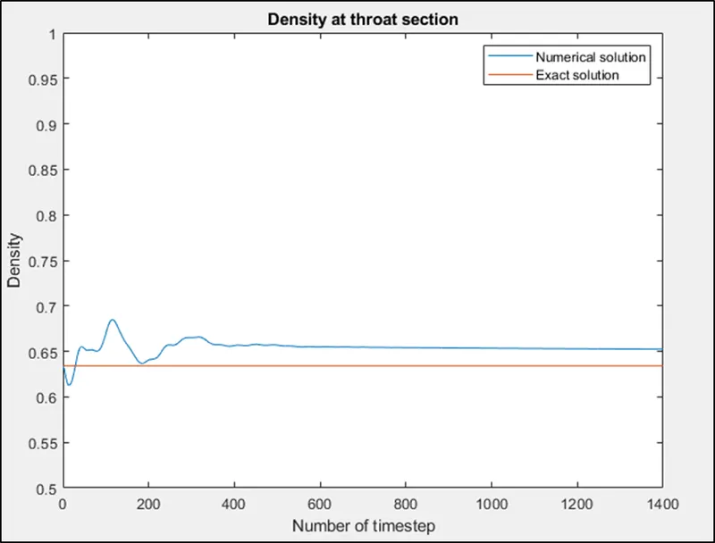
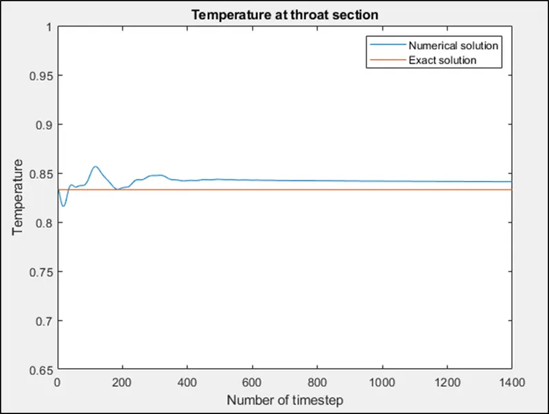
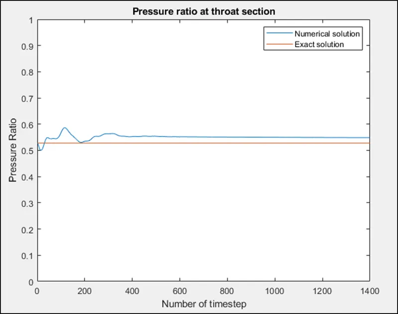
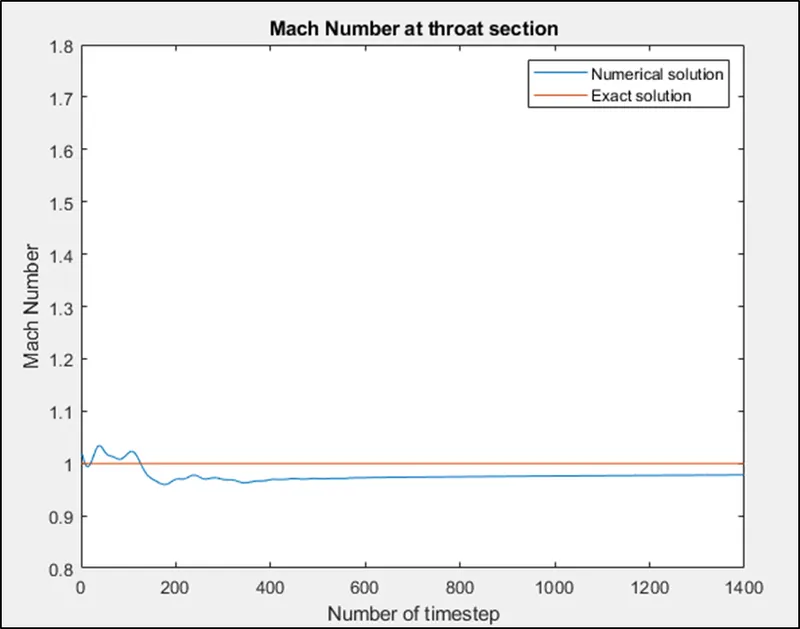
In the above four plots we can observe the time-wise variation of density,temperature,Pressure and mach number at the nozzle throat v/s the number of time steps.The red line in the plot represents exact,analytical values as obtained.We can observe from the plots that the numerical time-marching procedure converges to the proper theoretical steady-state answer.

• GRID INDEPENDENCE TEST:

FOR n=31

FOR n=61

COMPARISION:

	`rho^ast/rho_0`	`T^ast/T_0`	`p^ast/p_0`	M
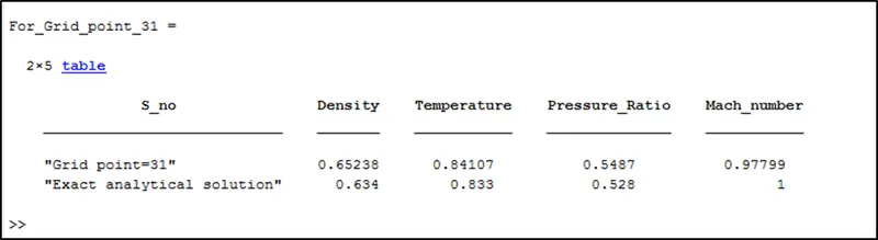
31 points	0.652	0.841	0.548	0.977
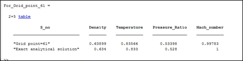
61 points	0.638	0.835	0.533	0.997
Exact analytical solution	0.634	0.833	0.528	1.000

Table compares the steady-state results of density,temperature,pressure and mach number at the throat for both the cases using 31 and 61 grid points and also compares with the exact analytical solution ,we observe that by doubling the number of grid points numerical soution improves marginally,so we can conclude that our original calculation using 31 grid points is essentially grid-independent.

• COMPARISION OF CONSERVATION AND NON-CONSERVATION FORM:

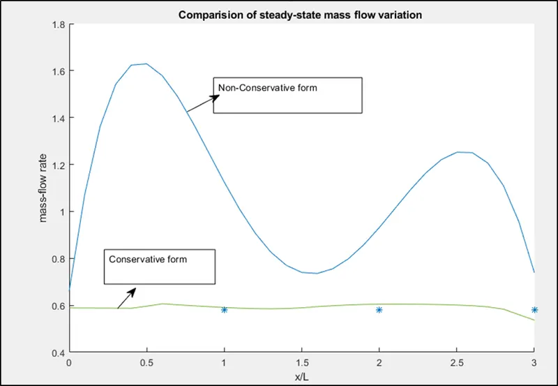
The plot shows the detailed comparision of the steady-state mass flow variation obtained with the nonconservation and conservation forms of the governing flow equations.

From the plot we can observe that the conservation form gives a distribution that is much closer to being a constant and the non-conservation results have sizeable variations,with oscilaations at the both inflow and outflow boundaries.The steady-state mass flow results obtained with the conservation form are,on the whole,much closer to the exact analytical solution shown by(****) in the plot.

	`rho^ast/rho_0`	`T^ast/T_0`	`p^ast/p_0`	M
Exact analytical solution	0.634	0.833	0.528	1.000
Non-conservation form n=31	0.638	0.836	0.534	0.999
Conservation form n=31	0.652	0.841	0.548	0.977

Table shows the comparision of steady-state results of conservation and nonconservation forms

Let us take a look at primitive variables,the first row in the table gives the exact,analytical result.The second and third row gives the numerical results for non-conservation and conservation form respectively,we observe that non-conservation form results are distinctly closer to the exact values.

• CONCLUSION:

1. The conservation form does a better job of preserving mass throughout the flow field,mainly because the mass flow itself is one of the dependent variable in the equations.In contrast,the dependent variables in the nonconservation form of the equation are the primitive variables,and mass flow is obtained only as secondary result.
2. There is no clear superiority of either form in terms of accuracy of the results.The non-conservation forms seems to produce slightly more accurate results for the primitive variables,and the conservation form seems to produce slightly more accurate results for the flux variables.
3. Comparing the amount of calculational effort to achieve a solution,we observe that the solution of the conservation form requires marginally more work.