Mixing Tee Simulation

Given:

• Simulate flow through mixing tee (short and long)
• Set up steady-state simulations to compare the mixing effectiveness when hot inlet temperature is 36 degree celsius & the Cold inlet is at 19 degree celsius.
• Use the k-epsilon and k-omega SST model for the first case
• Based on your result and judgment use the more suitable model for further cases. Giving the reason for choosing a suitable model is compulsory.

Aim:

Simulate the two cases below:

Case 1

• Short mixing tee with a hot inlet velocity of 3m/s.
• Momentum ratio of 2, 4.

Case 2

• Long mixing tee with a hot inlet velocity of 3m/s.
• Momentum ratio of 2, 4.

Where, Momentum ratio = velocity at cold inlet / velocity at hot inlet

In a table, compare the following values from the 2 cases:

1. Cell count
2. Average outlet temperature
3. Number of iterations for convergence

Additional results:

1. Velocity and temperature contour plots on the cut planes along and across the pipe.
2. Velocity and temperature line plots along and across the length of the pipe.
3. Perform Mesh independent study for any one case.
4. Discuss the effect of length and momentum ratio on results.

Introduction:

Mixing Tee:

Fluid mixing is represented in the form of mixing two coaxial jet flows with good mixing efficiency. It is generally used for applications that require an efficient mix of two fluid streams with different physical & chemical properties combined together to form one stream.

Application : used in high pressurised applications like an Air Conditioner.

Scope: This challenge helps us in investigating the mixing effectiveness by varying the length of tee and velocity at which the two fluids enter.

Turbulence:

It is caused by excessive kinetic energy in parts of a fluid flow, which overcomes the damping effect of the fluid's viscosity. For this reason turbulence is commonly realized in low viscosity fluids. In general terms, in turbulent flow, unsteady vortices appear of many sizes which interact with each other, consequently drag due to friction effects increases. This increases the energy needed to pump fluid through a pipe.

in general fluid flows turbulence is the norm and laminar flow is the exception. turbulence is a very complicated phenomenon, our understanding of which is very limited. thus when we try to model turbulence in a simulation there are various approaches that exist. it is on us to select a approach that works well with the physics of the problem.

Since the fluid mixing involves turbulence and to study the turbulence effect we use the K-epsilon turbulence model where we simulate the mean flow characteristics of the turbulent flow condition.

Realizable K- epsilon is used since it exhibits superior performance when flow involves rotation and boundary layers with adverse pressure gradients. It is effective for predicting the flow behavior at regions away from the wall.

Moreover, the standard deviation method is used to examine the mixing efficiency in tee simulation.

Reynolds averaged navier stokes equation:

The Reynolds-averaged Navier–Stokes equations (or RANS equations) are time-averaged equations of motion for fluid flow. The idea behind the equations is Reynolds decomposition, whereby an instantaneous quantity is decomposed into its time-averaged and fluctuating quantities.The RANS equations are primarily used to describe turbulent flows. These equations can be used with approximations based on knowledge of the properties of flow turbulence to give approximate time-averaged solutions to the Navier–Stokes equations.

K epsilon:

It is a two equation RANS turbulence model, in this model we solve for two variables, turbulent kinetic energy k and turbulent dissipation of kinetic energy epsilon. This model uses wall functions to account for the fluid velocity in the viscous sublayer near the wall.

Main limitations for K-epsilon models are:

1. No-slip walls.
2. Adverse pressure gradients.

But various models in the K-epsilon model were developed to improve the performance of the K-epsilon model. They are Realizable K-epsilon model, RNG K-epsilon model.

K-omega:

It is another turbulence model where rate of dissipation of kinetic energy epsilon is replaced by omega. The main objective of this model is to account for near wall interactions more accurately than the K-epsilon model.

Limitations for K-omega:

1. Difficulty of convergence compared to K-epsilon
2. Sensitivity to initial conditions.

Due to these limitations the K-omega SST model was developed. This model is a hybrid of K-omega and K-epsilon model. This model is used mainly in aeronautics areas where freestream turbulence levels have to be addressed and it can also applied to the viscous affected region without further modification.

Convergence:

Since most fluid flow problems are of a non- linear nature, dealing with phenomena like turbulence, to solve such problems we use an iterative solver to continuously improve our solution till 'convergence ' is reached. when solving a problem with multiple iterations convergence becomes related to the accuracy of the solution. typically when assessing convergence for a steady-state CFD solution we need to keep in mind three major things, they are:

1. Residual values
2. Solution Imbalance
3. Observing quantities of interest

the criteria for convergence that is being applied is:

1. continuity
2. x- velocity
3. y- velocity
4. z-velocity
5. energy
6. turbulence related variable

Numerical solution for the outlet mixture:

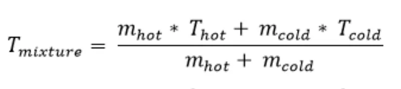
where

m=ρair⋅A⋅V

ρair=1.225Kg/m^3

Area of cold inlet=0.0002m^2

Area of hot let=0.0009m^2

For momentum ratio 2:

Tmixture=30.76 Celsius

For momentum ratio 4:

Tmixture=27.780 Celsius

SOLVING AND MODELLING APPROACH

The solving approach is represented as a workflow diagram are shown in the following steps:

1. Setup the geometry in Ansys workbench
2. Extract the fluid volume region.
3. Generate mesh for a correct sizing.
4. Set up post processing data and the required turbulence model.
5. Run the solver.
6. Check for convergence.
7. Post process the results

The flowchart for the above steps are shown below

Procedure (mostly same for each case with only inlet/outlet velocity and turbulence model changing):

1. Geometry preparation

• IMPORT GEOMETRY IN SPACECLAIM> PREPARE > VOLUME EXTRACTION > SELECT EDGES > CLICK TICK.
• THEN IN STRUCTURE > MIXING TEE SHORT > UNSELECT SHELL1 > SUPPRESS FOR PHYSICS > CLOSE GEOMETRY.

2. Mesh

• OPEN MESH >ENTITY SELECTION > FACE SELECTION > select the faces of the geometry to be mentioned as boundaries NAMELY INLET X,INLET Y,OUTLET AND WALLS
• MESH > DETAILS OF MESH > QUALITY > MESH METRIC > Select 'Element quality'.
• MESH > GENERATE MESH.
• Initially keep the geometry in Y-direction. Now by using SECTION PLANE BUTTON, click and drag at the center to foam a line, so that it cuts the geometry.

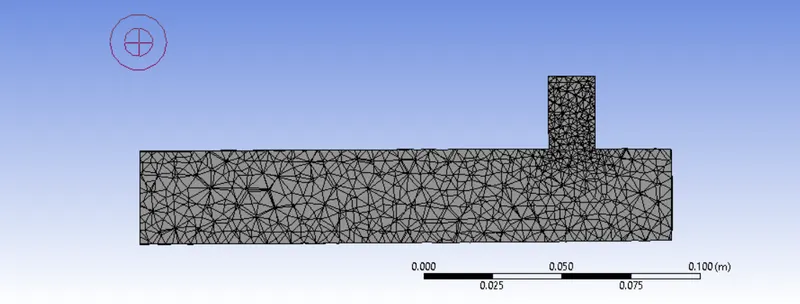
• Close the Mesh

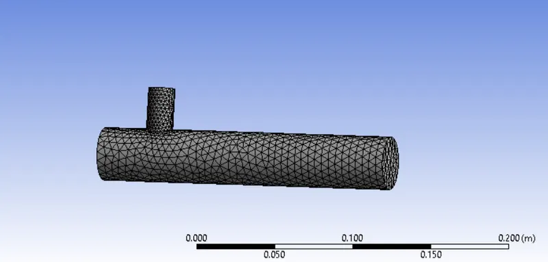
NOTE: AS LONG AS ELEMENT QUANTITY is not lower than 5%, SIMULAION RUNS

3. Set Up

• DOUBLE CLICK SETUP > FLUENT LAUNCHER >DOUBLE PRECISION AND 4 CORES.
• Ansys Fluent is opened.

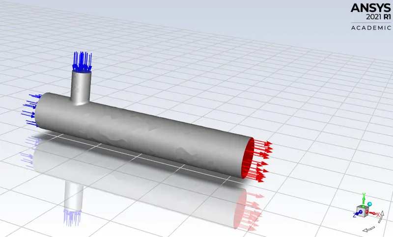
• In the Graphics window > GEOMETRY AND CONSOLE window is displayed.
• SETTING UP DOMAIN >MESH > select CHECK. Then in CONSOLE WINDOW it shows 'CHECKING MESH…. DONE'.
• To Change the Units, SETTING UP DOMAIN > click Units
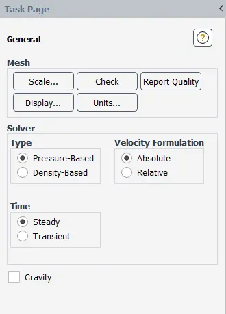
• SETTING UP PHYSICS > SOLVER > select Time = STEADY, Type = PRESSURE BASED & Velocity Formation = ABSOLUTE.

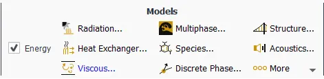
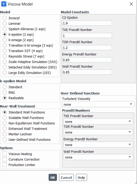
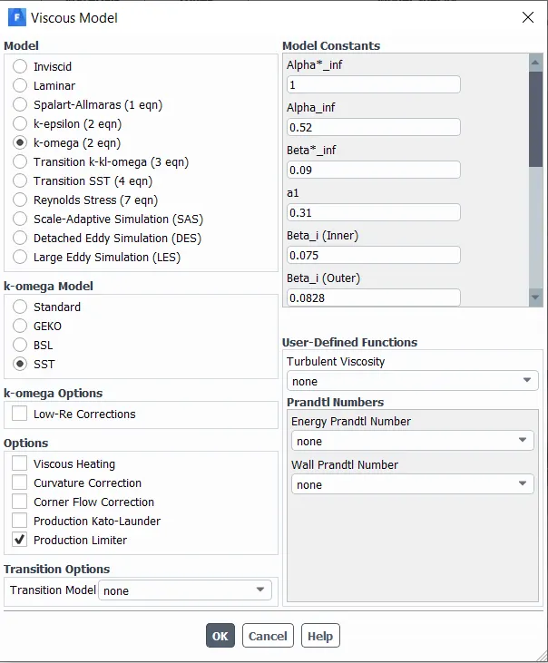
• SETTING UP PHYSICS > MODELS > select ENERGY. VISCOUS MODEL > Model > K-epsilon Model, REALIZABLE K-epsilon Model, STANDARD WALL FUNCTIONS >OK. OR K-Omega Model, SST K-epsilon Model, PRODUCTION LIMITER >OK, for K-Omega model.

• SETTING UP PHYSICS > BOUNDARIES > ASK PAGE opens. Enter the values for Momentum, Thermal for both 'inlet-x' and 'inlet-y'. Then click OK.

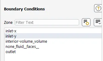
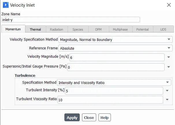
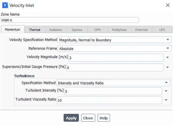
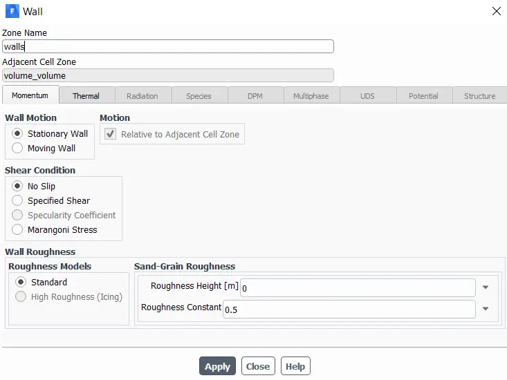
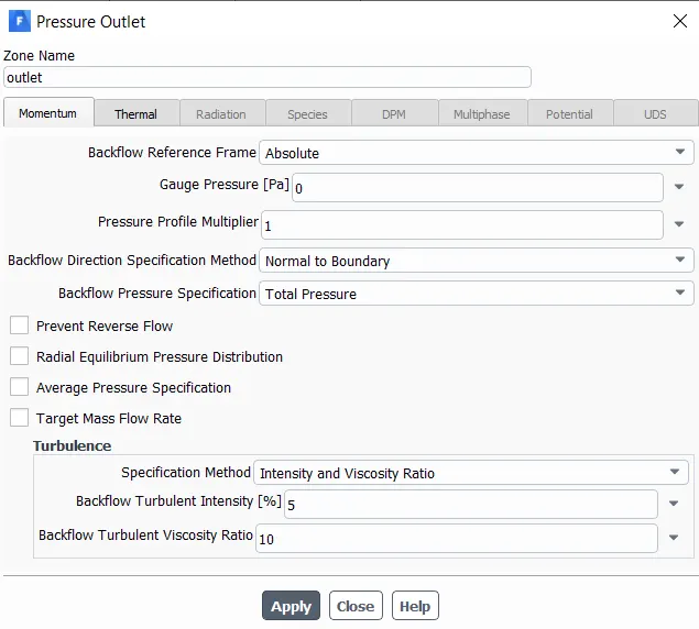
• FOR BOUNDARY 'outlet', the GAUGE PRESSURE (PASCAL) = 0 is available by default > Click OK.

4. Solution

• SOLVING > CONTROLS, REPORTS, INITIALIZATION, RUN CALCULATION.
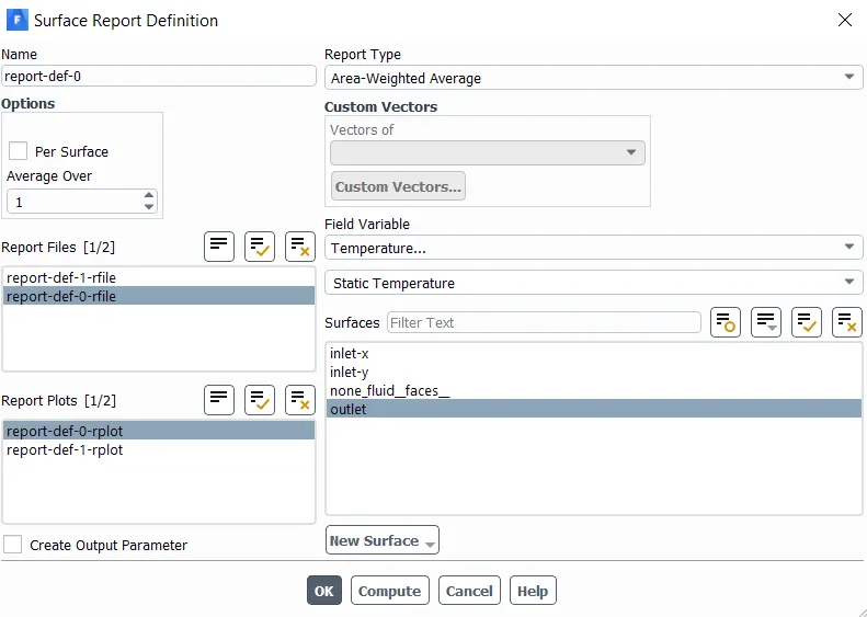
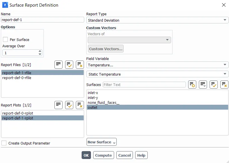
• REPORTS > DEFINITIONS > NEW > SURFACE REPORT >AREA WEIGHTED AVERAGE. Similarly, select 'STANDARD DEVIATION', For both the cases > a 'SURFACE REPORT DEFINITION WINDOW' pops up > select the FIELD VARIABLE = Temperature
• CREATE > select REPORT FILE and REPORT PLOT.

• INITIALIZATION > select METHOD = HYBRID > click t=0 INITIALIZE

• RUN CALCULATION > NO. OF ITERATIONS =300 and press CALCULATE.

5. Results and Discussion:

• Double click on RESULTS > Post process window opens
• volume_volume > select 'wall volume_volume' and hide all inlets and outlets
• Plane Creation > Top Toolbar > INSERT > LOCATION > PLANE
• Plane 1 > Double click > COLOR > Mode = VARIABLE > In VARIABLE > select TEMPERATURE > Apply
• Similarly make another plane accross the pipe.

Observation:

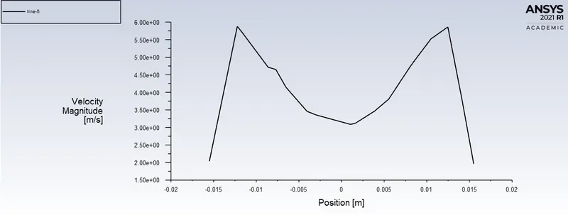
Cell Count In CASE-1 = 12,657

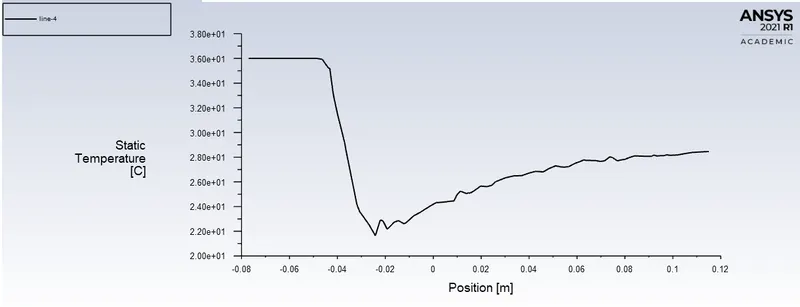
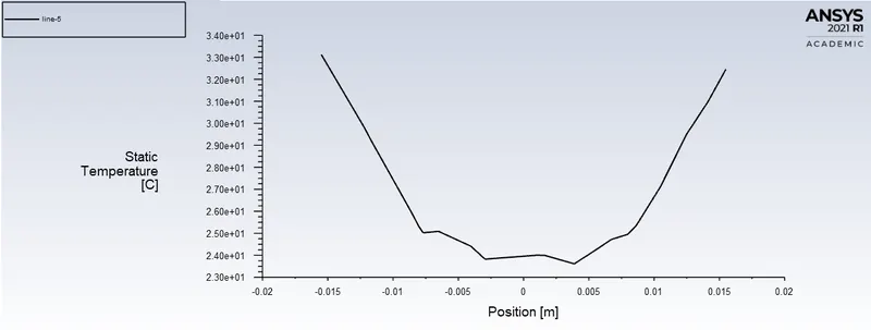
case 1(MR=2, VM=k-epsilon)

1. Average outlet temperature =30.25 degree celcius
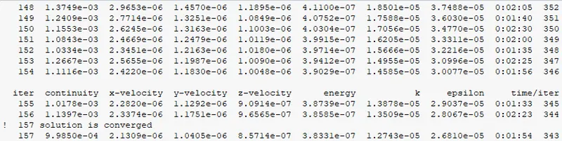
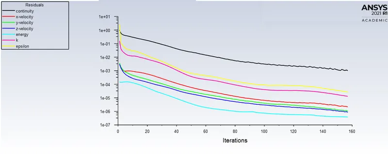
2. Number of iterations for convergence = 157

STD. deviation of temperature graph:

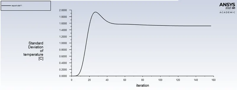
std. deviation value from graph: 1.518 degree celcius

Area weighted average of temperature:

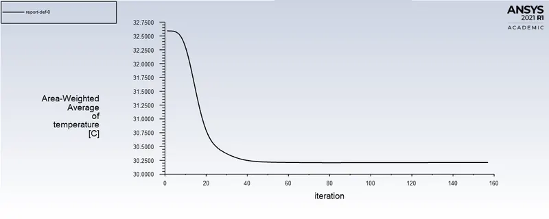
avg. temp value from graph: 30.211 degree celcius

theoritical value, Tmixture=30.76 Celsius

error=0.549 celcius

Residual convergence plot:

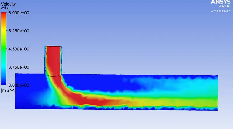
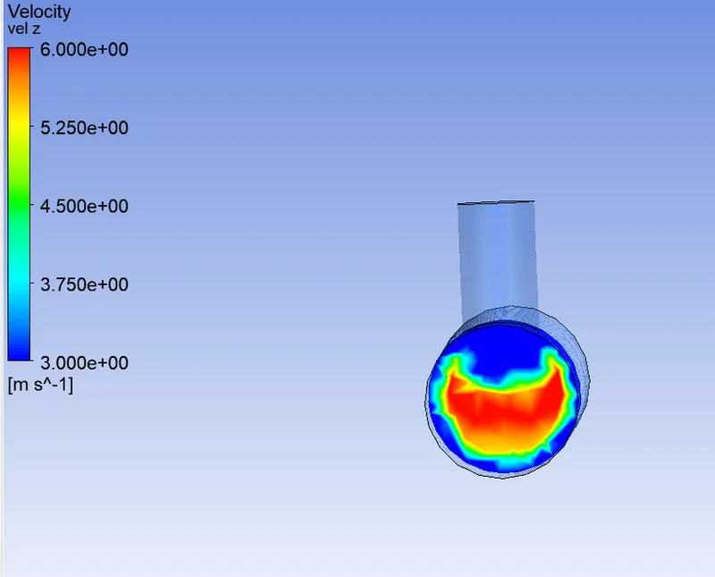
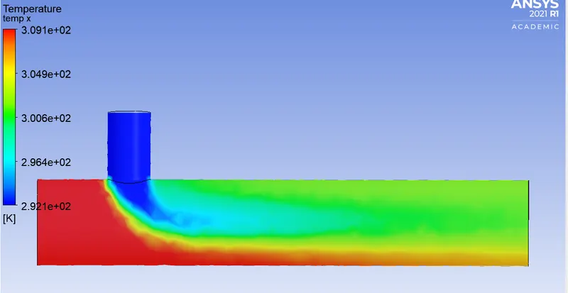
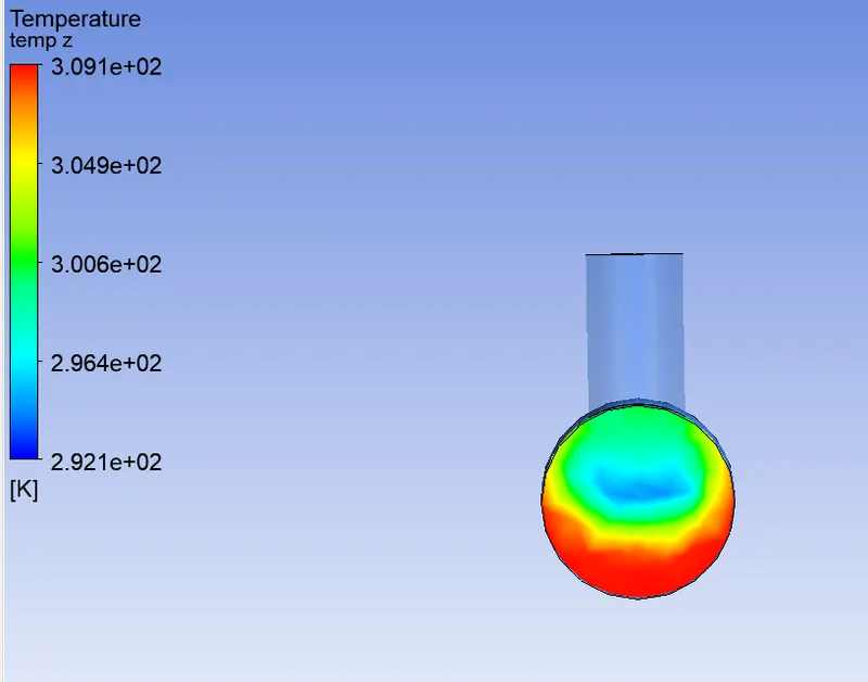
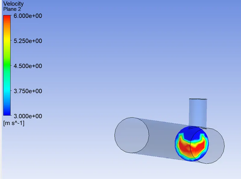
Velocity and temperature contour plots on the cut planes along and across the pipe.

velocity contour plots:

Temperature contour plots

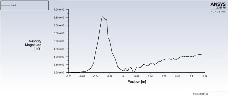
Velocity and temperature line plots along and across the length of the pipe.

Velocity line plots

Along the length

Across the length

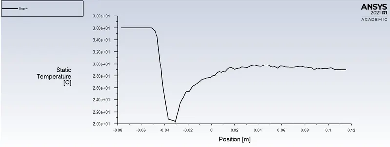
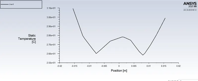
temperature line plots

Along the length

Across the length

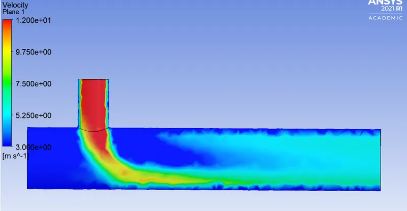
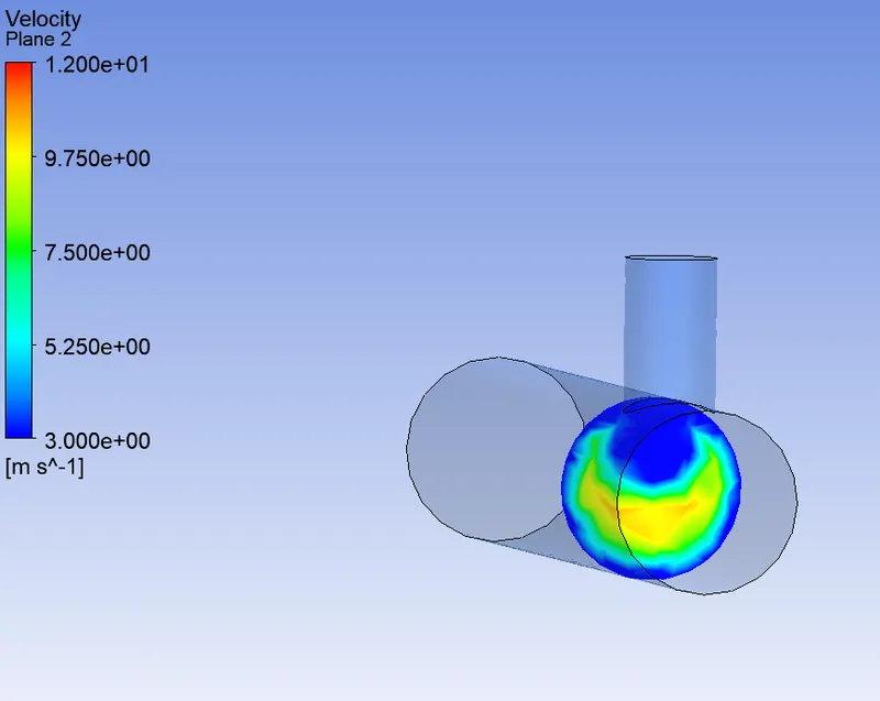
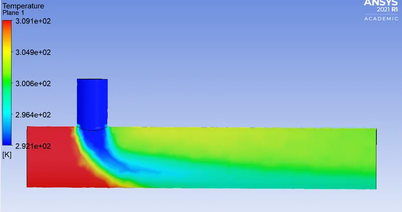
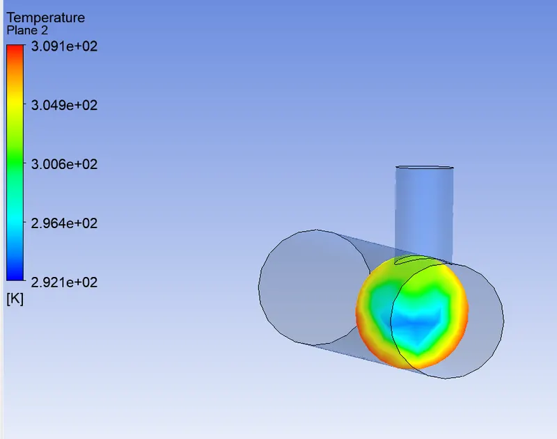
case 1(MR=4, VM=k-epsilon)

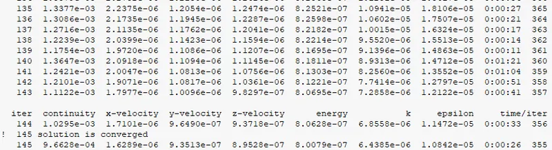
1. Average outlet temperature = 27.55 degree celcius
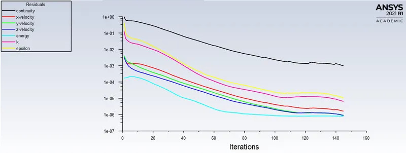
2. Number of iterations for convergence = 145

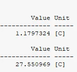
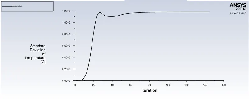
STD. deviation of temperature graph:

value on graph:1.179 degree celcius

Area weighted average of temperature:

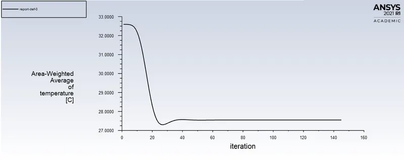
Average outlet temperature = 27.55 degree celcius

theoritical value, Tmixture=27.780 degree Celsius

error=0.23 degree celcius

Residual convergence plot:

Velocity and temperature contour plots on the cut planes along and across the pipe.

velocity contour plots:

Temperature contour plots

Velocity and temperature line plots along and across the length of the pipe.

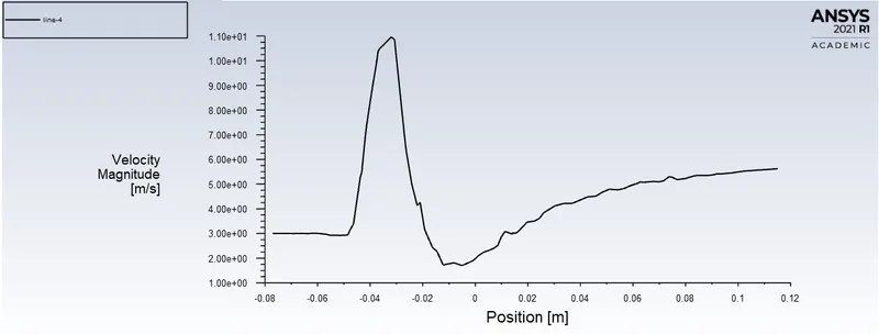
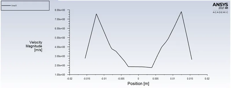
Velocity line plots

Along the length

Across the length

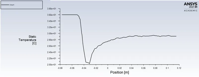
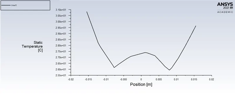
temperature line plots

Along the length

Across the length

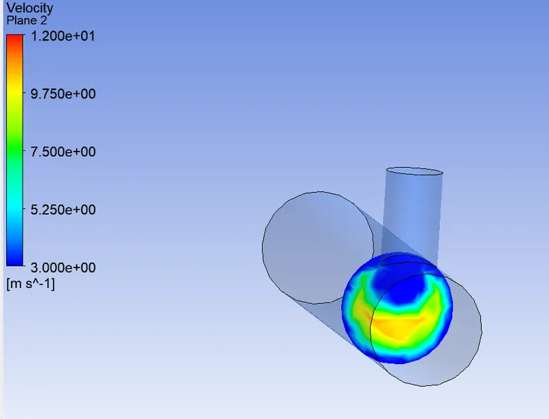
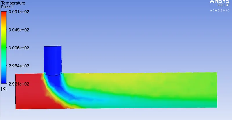
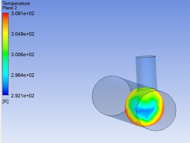
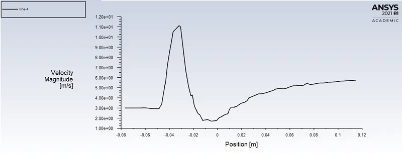
case 1(MR=4, VM=k-omega)

1. Average outlet temperature = 27.53 degree celcius
2. Number of iterations for convergence = 147

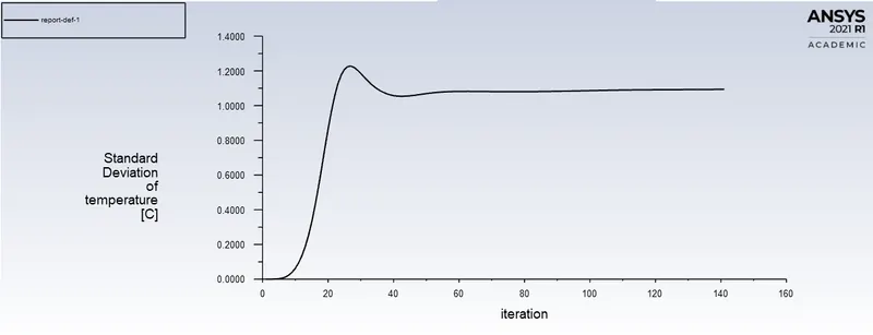
STD. deviation of temperature graph:

value on graph:1.093 degree celcius

Area weighted average of temperature:

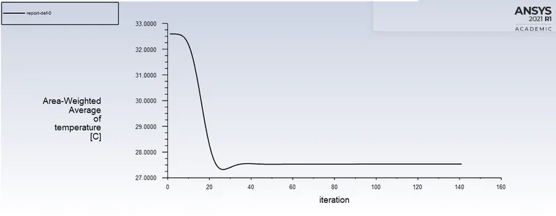
Average outlet temperature = 27.53 degree celcius

theoritical value, Tmixture=27.780 degree Celsius

error=0.25 degree celcius

note:slightly bigger margin in error as compared to kepsilon turbulence model.

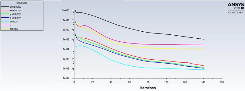
Residual convergence plot:

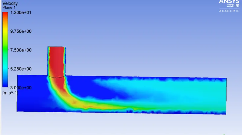
Velocity and temperature contour plots on the cut planes along and across the pipe.

velocity contour plots:

Temperature contour plots

Velocity and temperature line plots along and across the length of the pipe.

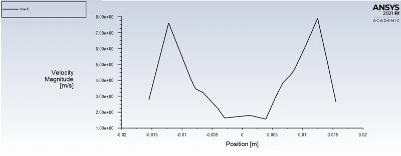
Velocity line plots

Along the length

Across the length

temperature line plots

Along the length

Across the length

Main difference

The k- omega model is well suited for simulating flow in the viscous sub-layer. On the contrary, The k-epsilon model is ideal for predicting flow in the regions away from the wall

The SST model exhibit less sensitivity to free stream conditions (Flow outside the boundary layer) than many other turbulence models.

The shear stress limiter helps the k-omega model avoid a build-up of excessive turbulent kinetic energy near stagnation points.

Although, in the above cases, the results are pretty much identical(slightly larger error in average temperature value in k-omega model), but since we're not interested in simulation results near the walls, we will with go with k-epsilon model for more reliable results in further simulations.

Now, let us conduct our simulation further with k-epsilon model.

Cell Count In CASE-2 = 32330

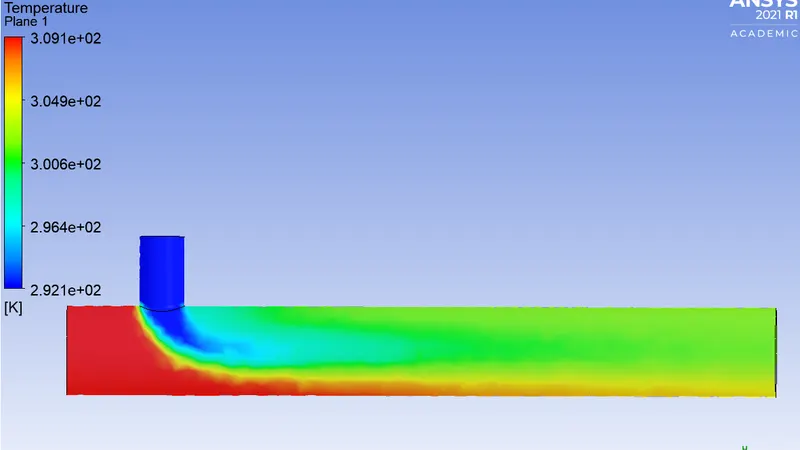
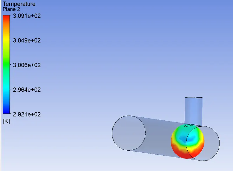
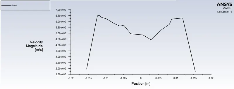
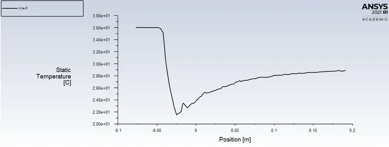
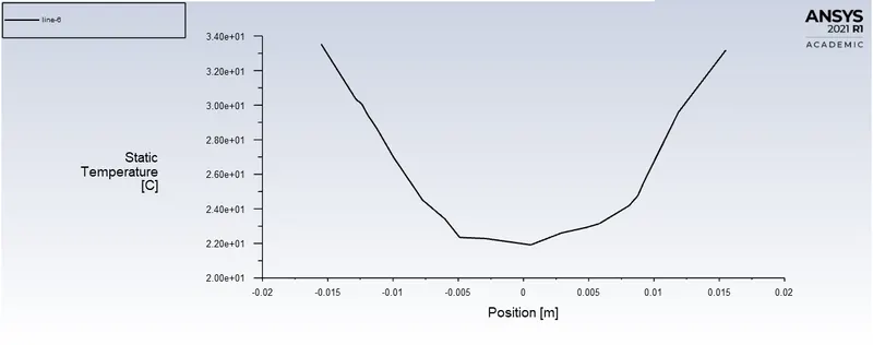
case 2(MR=2, VM=k-epsilon)

1. Average outlet temperature = 30.288 degree celcius
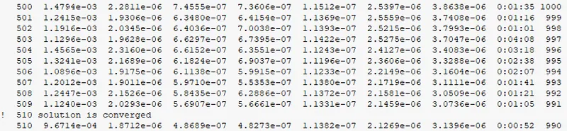
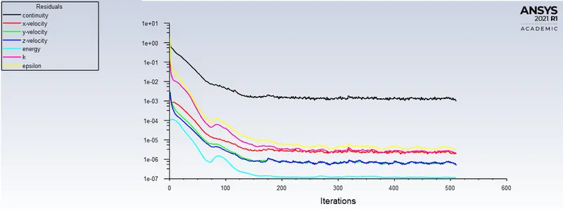
2. Number of iterations for convergence = 510

STD. deviation of temperature graph:

value from graph: 1.11 degree celcius

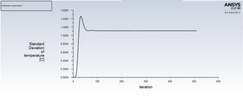
Area weighted average of temperature:

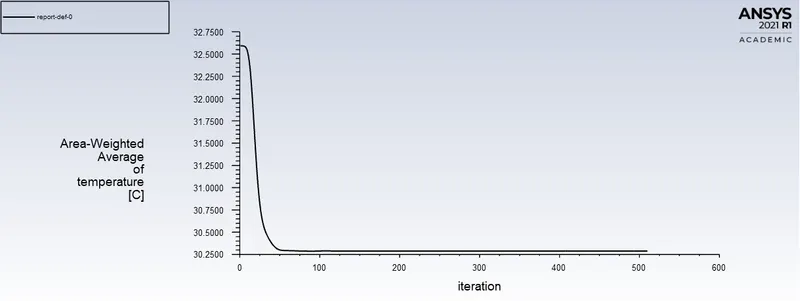
Average outlet temperature = 30.288 degree celcius

theoritical value, Tmixture=30.76 degree Celsius

error=0.48 degree celcius

Residual convergence plot:

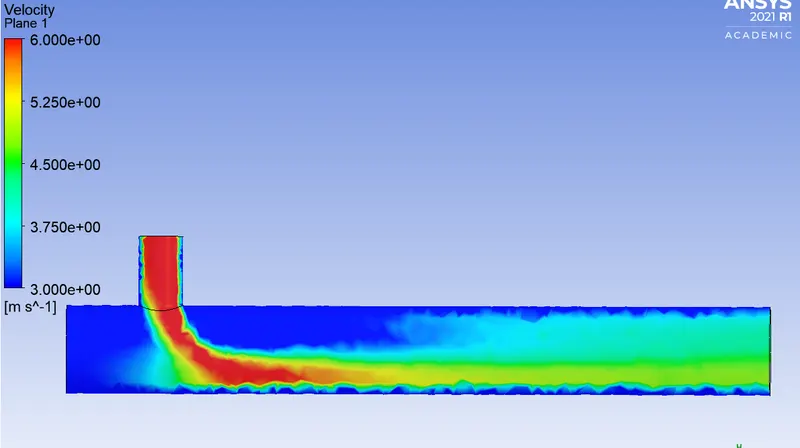
Velocity and temperature contour plots on the cut planes along and across the pipe.

velocity contour plots:

Temperature contour plots

Velocity and temperature line plots along and across the length of the pipe.

Velocity line plots

Along the length

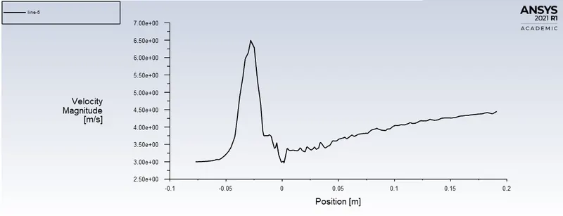
Across the length

temperature line plots

Along the length

Across the length

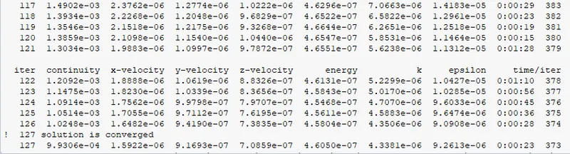
case 2(MR=4, VM=k-epsilon)

1. Average outlet temperature = 27.489 degree celcius
2. Number of iterations for convergence = 127

STD. deviation of temperature graph:

value from graph: 0.651 degree celcius

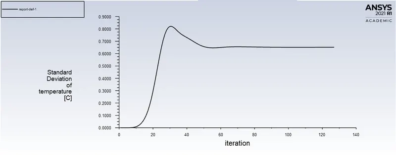
Area weighted average of temperature:

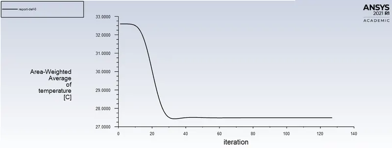
Average outlet temperature = 27.489 degree celcius

theoritical value, Tmixture=27.78 degree Celsius

error=0.291 degree celcius

Residual convergence plot:

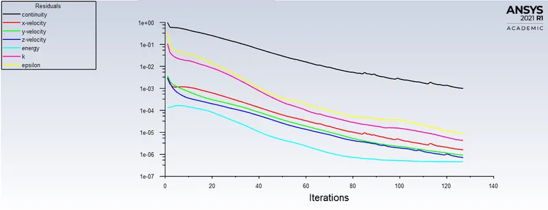
Velocity and temperature contour plots on the cut planes along and across the pipe.

velocity contour plots:

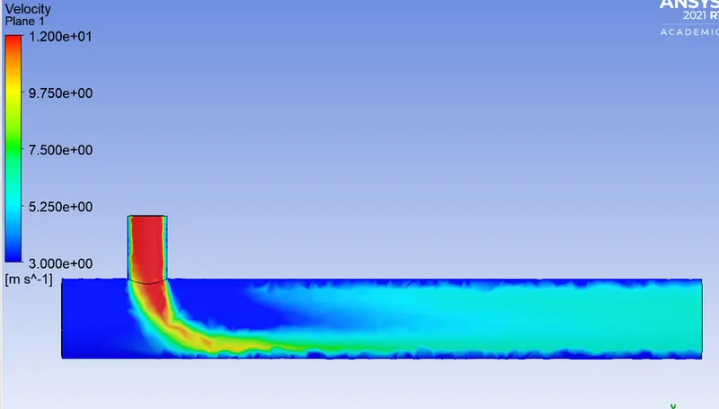
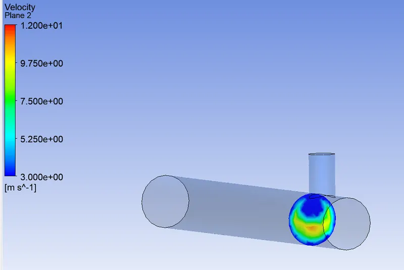
Temperature contour plots

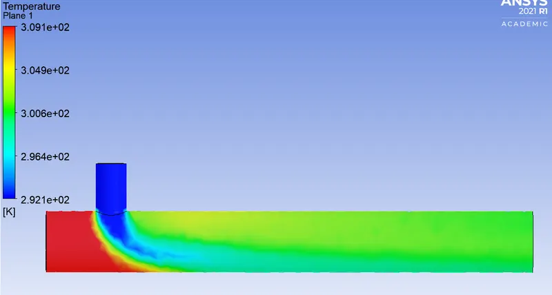
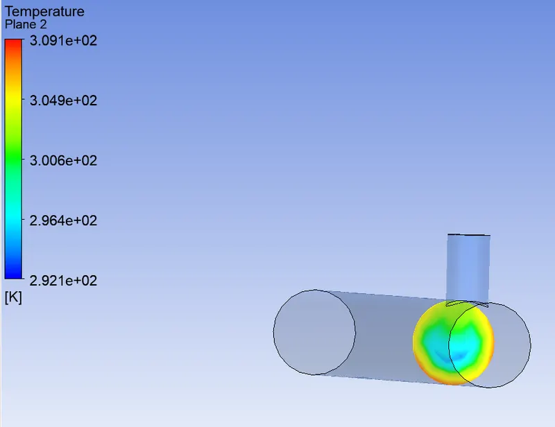
Velocity and temperature line plots along and across the length of the pipe.

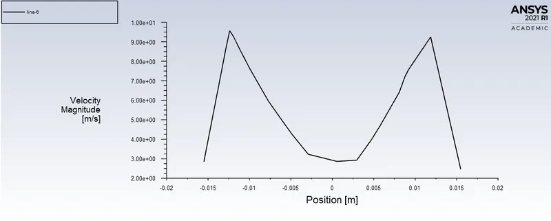
Velocity line plots

Along the length

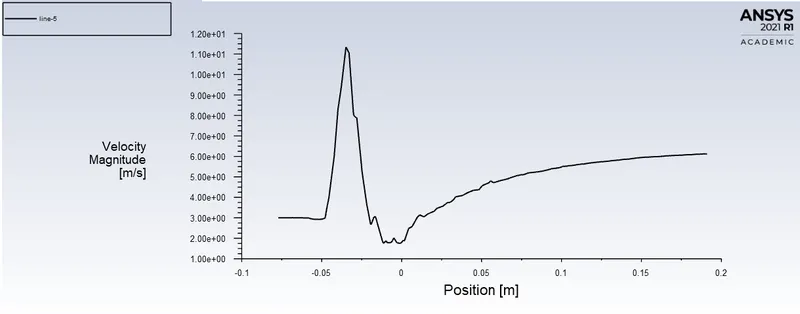
Across the length

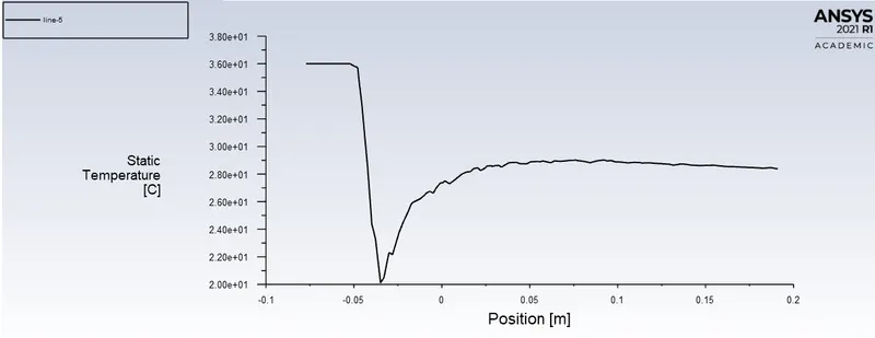
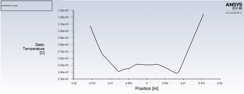
temperature line plots

Along the length

Across the length

Mesh independent study on case-1 (mesh element size = 0.003m; Cell Count In CASE-1, mr-2 = 82,882 )

A mesh independence (or grid independence) study is something an analyst can perform to determine the dependence of the results on the mesh density.

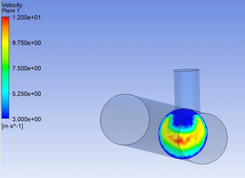
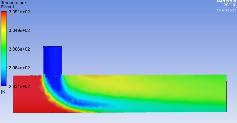
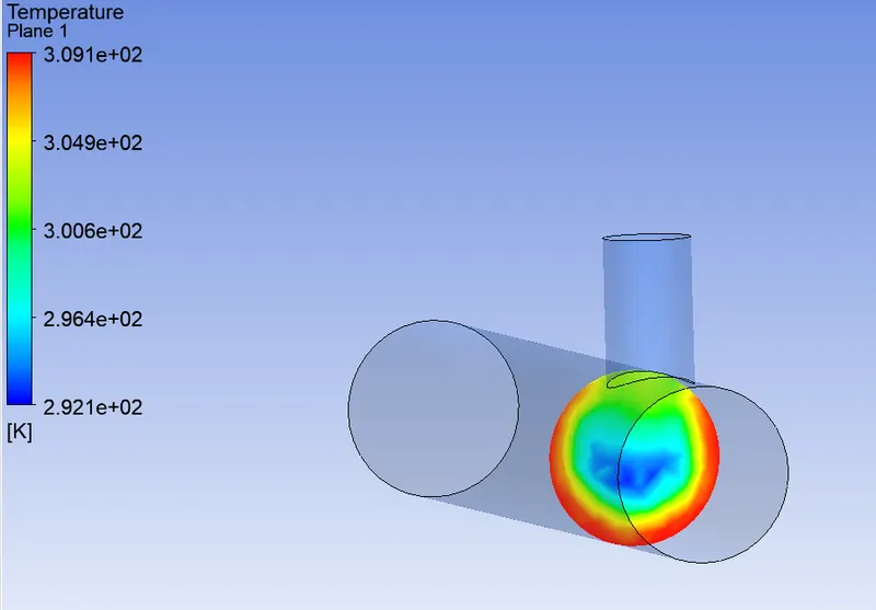
case 1(MR=4, VM=k-epsilon)

1. Average outlet temperature = 27.631 degree celcius
2. Number of iterations for convergence =144

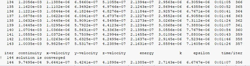
STD. deviation of temperature graph:

value from graph=1.06 degree celcuis

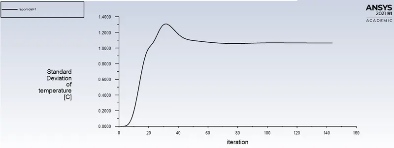
Area weighted average of temperature:

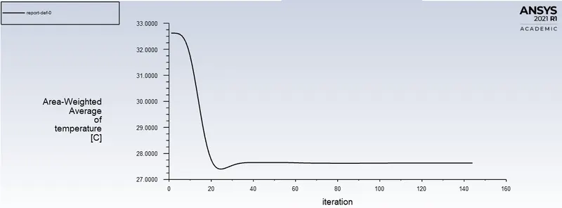
Average outlet temperature = 27.631 degree celcius

theoritical value, Tmixture=27.78 degree Celsius

error=0.149 degree celcius

Residual convergence plot:

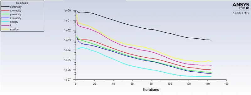
Velocity and temperature contour plots on the cut planes along and across the pipe.

velocity contour plots:

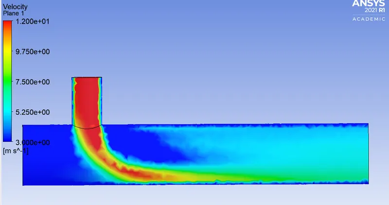
Temperature contour plots

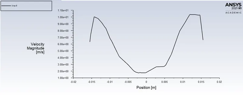
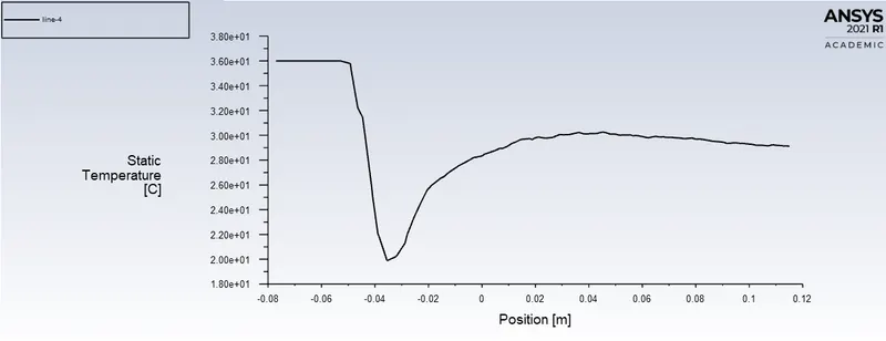
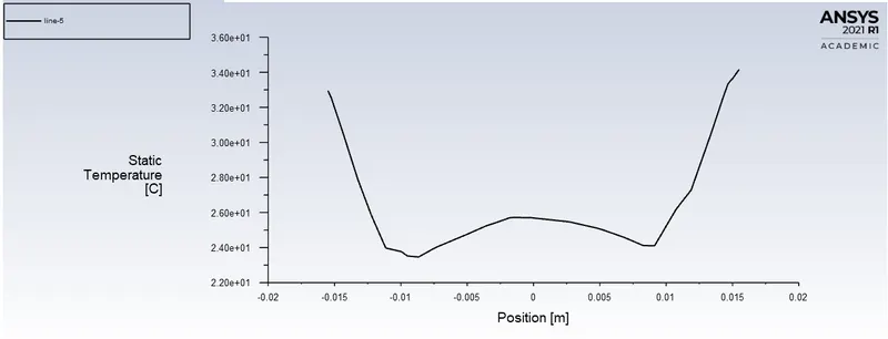
Velocity and temperature line plots along and across the length of the pipe.

Velocity line plots

Along the length

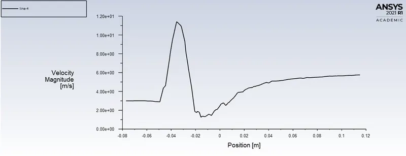
Across the length

temperature line plots

Along the length

Across the length

Discussion:

The effect of length and momentum ratio on results:

case 1: the higher momentum-ratio gave lower average temperature and lower temperature deviation(lower deviation meaning better mixing of hot and cold air)

case 2: in case 2, the effect of momentum-ratio on temperature and mixing of hot air, was same as that in case 1. However, due to longer diffusion period in case 2, the longer length of pipe meant lower temperature deviation at outlet(better mixing), and lower average temperature as compared to short pipe (also closer to theoritical values of temperature at different momentum ratios).

Effect of turbulence model on results:

Between k-epsilon and k-omega, they both beared the same results, however average temperature in k-epsilon was closer to that of theoritical value.

But the main reason we cho0se k-epsilon in such simulation, is because we're not interested in simulation of air near the walls of the pipe, but we're interested in simulations away from it, in which case k-epsilon bears more reliable results.

Effect of mesh on results:

By making the mesh finer, we can get more accurate results, as comparing the results of simulation with lower mesh cells with that of higher mesh cells, in case one ( short pipe with MR=4) the results came out to be better in the simulation in higher mesh cells with, lower temperature deviation and average temperature value closer to the theoritical value.

Conclusion:

• To get better mixing results at outlet, high velocity of flow from inlet(higher momentum ratio) is very effective. Therefore, a higher momentum ratio gives better mixing of hot and cold fluid stream at the outlet.
• Due to higher diffusion, the longer Length of the mixing tee always gives slightly better mixing of two-fluid.
• k-epsilon models predict flow virtually far from the boundaries (wall), and the k-omega model predicts near the wall. As in this case we need a flow simulation turbulent model far from the wall, therefore, the k-epsilon method is used.
• In mesh independence test, the finer the mesh the accurate the results are.
• Finally, in the above cases, it is very important to use a short mixing tee with a momentum ratio of 4 to get precise results but one has to consider the diffusion of flow along the length of the mixing tee, a long mixing tee with momentum will be the greater option.