Week 7 - Simulation of a 1D Super-sonic nozzle flow simulation using Macormack Method
** Code of Non-Conservative
clc
clear all
close all

%% Create 1D domain
n=31;
L=3;
x=linspace(0,L,n);
dx=x(2)-x(1);
th=(n-1)/2;       % Location of throat
%% Constants
gama=1.4;

%% Time steps
nt=1800;
dt=0.01;

%% initial values of properties
rho=1-0.3146*x;                  % Density
t=1-0.2314*x;                    % Temperature
v=(0.1+1.09*x).*t.^0.5;          % Velocity
a=1+2.2*(x-1.5).^2;              % Area

%% CFL number
cfl=max((v+sqrt(t))*dt/dx);

%% Loop counter
iteration=0;
%% Loops
for k=1:nt   % Time loops
    %% Storing old values

    rho_old = rho;
    t_old = t;
    v_old = v;

    % Predictor step
    for j=2:n-1
        dvdx= (v(j+1)-v(j))/dx;
        dlogadx=(log(a(j+1))-log(a(j)))/dx;
        drhodx=(rho(j+1)-rho(j))/dx;
        dtdx=(t(j+1)-t(j))/dx;

        % Continuity Equation
        drhodt_p(j)=-rho(j)*dvdx -rho(j)*v(j)*dlogadx-v(j)*drhodx;

        % Momentum Equation
        dvdt_p(j)=-v(j)*dvdx-(1/gama)*(dtdx+(t(j)/rho(j))*drhodx);

        % Energy Equation
        dtdt_p(j)=-v(j)*dtdx-(gama-1)*t(j)*(dvdx+v(j)*dlogadx);

        % Solution update
        v(j)=v(j)+dvdt_p(j)*dt;
        rho(j)=rho(j)+drhodt_p(j)*dt;
        t(j)=t(j)+dtdt_p(j)*dt;
    end

    % Corrector step
    for i=2:n-1
        dvdx= (v(i)-v(i-1))/dx;
        dlogadx=(log(a(i))-log(a(i-1)))/dx;
        drhodx=(rho(i)-rho(i-1))/dx;
        dtdx=(t(i)-t(i-1))/dx;

        % Continuity Equation
        drhodt_c(i)=-rho(i)*dvdx -rho(i)*v(i)*dlogadx-v(i)*drhodx;

        % Momentum Equation
        dvdt_c(i)=-v(i)*dvdx-(1/gama)*(dtdx+(t(i)/rho(i))*drhodx);

        % Energy Equation
        dtdt_c(i)=-v(i)*dtdx-(gama-1)*t(i)*(dvdx+v(i)*dlogadx);
    end

    % Average
    dvdt=0.5*(dvdt_p+dvdt_c);
    drhodt=0.5*(drhodt_p+drhodt_c);
    dtdt=0.5*(dtdt_p+dtdt_c);

    %% Apply boundary condition
    % Inlet:
    v(1)=2*v(2)-v(3);

    % Outlet:
    v(n)=2*v(n-1)-v(n-2);
    rho(n)=2*rho(n-1)-rho(n-2);
    t(n)=2*t(n-1)-t(n-2);

    %% Final Solution updating
    for m=2:n-1
        rho(m)=rho_old(m)+drhodt(m)*dt;
        v(m)=v_old(m)+dvdt(m)*dt;
        t(m)=t_old(m)+dtdt(m)*dt;
    end
    iteration=iteration+1;
    % Pressure
    p=rho.*t;
    % MACH NUMBER
    mach=v./sqrt(t);
    % Mass Flow rate
    m=rho.*a.*v;
    %% Plotting
    figure(1)
    plot(x,v,'color','r')
    title(sprintf('Iteration=%d',iteration))
    xlabel('Nozzle Length')
    ylabel('Velocity')
    grid on


    figure(2)
    plot(x,m,'color','g','linewidth',2)
    xlabel('Nozzle Length')
    ylabel('Mass Flow Rate')
    title(sprintf('Iteration=%d',iteration))

    figure(3)
    plot(x,rho,'color','b')
    title(sprintf('Iteration=%d',iteration))
    xlabel('Nozzle Length')
    ylabel('Density')
    grid on


    figure(4)
    plot(x,t,'color','g')
    title(sprintf('Iteration=%d',iteration))
    xlabel('Nozzle Length')
    ylabel('Temperature')
    grid on

    %% Time wise variation plots
    % Mass flow rate
    figure(5)
    hold on
    if k==1
        plot(x,rho)
        xlabel('Nozzle Length')
        ylabel('density')
    end
    if k==250
        plot(x,rho)
        xlabel('Nozzle Length')
        ylabel('density')
    end
    if k==500
        plot(x,rho)
        xlabel('Nozzle Length')
        ylabel('density')
    end
    if k==750
        plot(x,rho)
        xlabel('Nozzle Length')
        ylabel('density')
    end
    if k==1000
        plot(x,rho)
        xlabel('Nozzle Length')
        ylabel('density')
    end
    if k==1500
        plot(x,rho)
        xlabel('Nozzle Length')
        ylabel('density')
    end
    if k==1800
        plot(x,rho)
        xlabel('Nozzle Length')
        ylabel('density')
    end
    legend('t=0.01','t=2.5','t=5','t=7.5','t=10','t=15','t=18')

    figure(6)
    hold on
    if k==1
        plot(x,t)
        xlabel('Nozzle Length')
        ylabel('temperature')
    end
    if k==250
        plot(x,t)
        xlabel('Nozzle Length')
        ylabel('temperature')
    end
    if k==500
        plot(x,t)
        xlabel('Nozzle Length')
        ylabel('temperature')
    end
    if k==750
        plot(x,t)
        xlabel('Nozzle Length')
        ylabel('temperature')
    end
    if k==1000
        plot(x,t)
        xlabel('Nozzle Length')
        ylabel('temperature')
    end
    if k==1500
        plot(x,t)
        xlabel('Nozzle Length')
        ylabel('temperature')
    end
    if k==1800
        plot(x,t)
        xlabel('Nozzle Length')
        ylabel('temperature')
    end
    legend('t=0.01','t=2.5','t=5','t=7.5','t=10','t=15','t=18')

    %% Storing values at throat
    rho_th(k)=rho(th);       % Density at throat
    v_th(k)=v(th);           % Velocity at throat
    t_th(k)=t(th);           % Temperature at throat
    p_th(k)=p(th);           % Pressure at throat
    mach_th(k)=mach(th);     % Mach number at throat
    m_th(k)=m(th);           % Mass flow rate at throat
end

figure(7)
subplot(6,1,1)
plot(v_th)
xlabel('Iteration')
ylabel('Velocity')
title('Velocity variation at throat with time')

subplot(6,1,2)
plot(rho_th)
xlabel('Iteration')
ylabel('Density')
title('Density Variation at throat with time')

subplot(6,1,3)
plot(t_th)
xlabel('Iteration')
ylabel('Temperature')
title('Temperature variation at throat with time')

subplot(6,1,4)
plot(p_th)
xlabel('Iteration')
ylabel('Pressure')
title('Pressure Variation at throat with time')

subplot(6,1,5)
plot(mach_th)
xlabel('Iteration')
ylabel('Mach Number')
title('Mach Number variation of Flow at throat at time')

subplot(6,1,6)
plot(m_th)
xlabel('Iteration')
ylabel('Mass Flow rate')
title('Mass flow rate variation at throat with time')

figure(8)
plot(m)
xlabel('Nozzle Length')
ylabel('Mass Flow rate')
title('Mass flow rate')
# Results:
A. Steady state premitive variables
1. Velocity
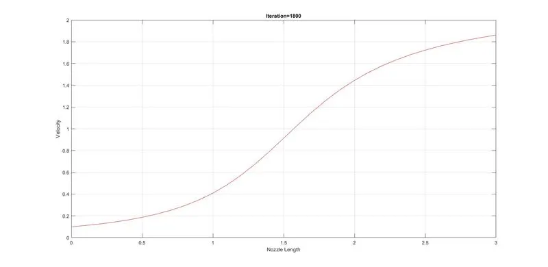
From figure, it can be observed that velocity is increasing towards the end. So flow is accelerating.
2. Density
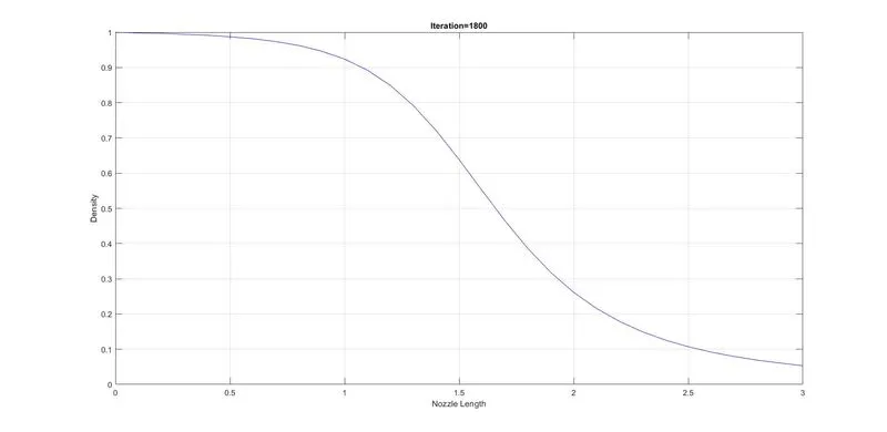
From above figure, it is seen that the density is reducing. The reduction in density indicate the acceleration of flow due to expansion.
3. Mass flow rate
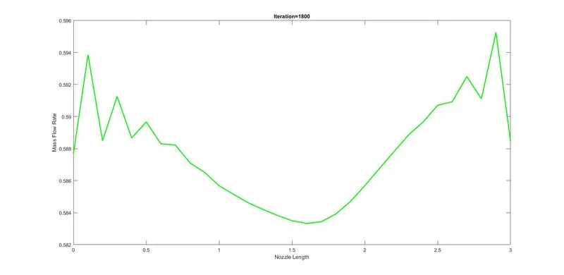
At throat, area is minimum and hence mass flow rate is also minimum. The mass flow rate is reducing from inlet to throat and then it is increading from throat to outlet.
4. Temperature
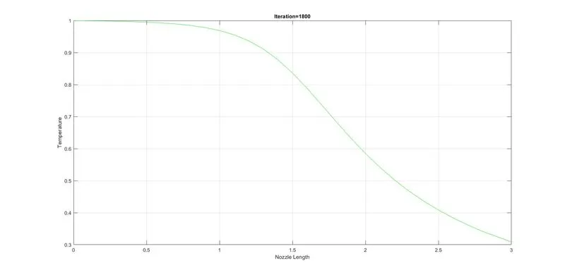
The temperature is reducing from inlet to outlet. This shows adiabatic expansion of flow through nozzle.
B. Time wise variation of primitive variables
1. Velocity
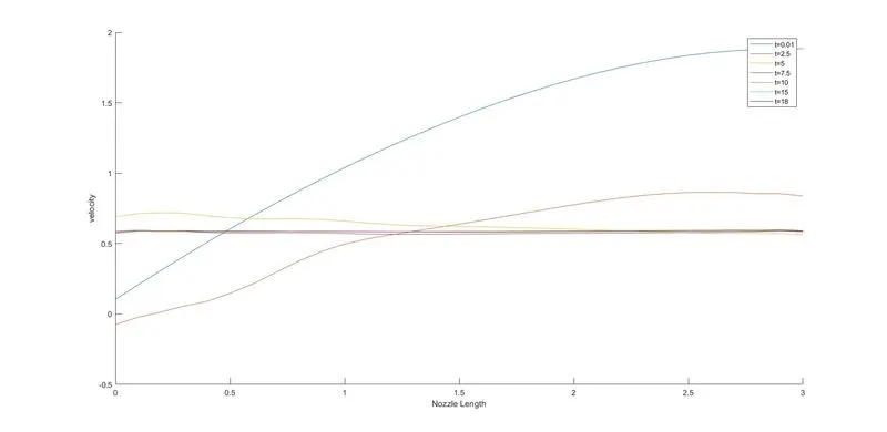
The above graph shows that steady state is achieved after t=10 sec, because velocity profile is nearly same.
2. Density
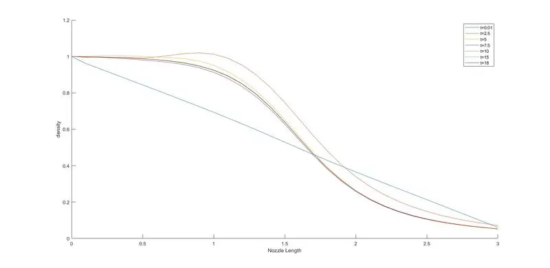
The above graph shows that steady state is achieved after t=10 sec, because density profile is nearly same.
3. Mass flow rate
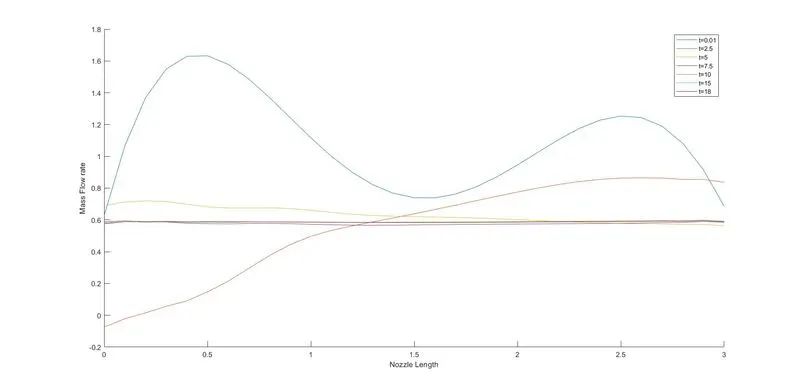
The above graph shows that steady state is achieved after t=10 sec, because mass flow rate profile is nearly same.
4. Temperature
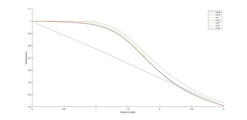
The above graph shows that steady state is achieved after t=10 sec, because temperature profile is nearly same.
C. Time wise variation of variables inside nozzle
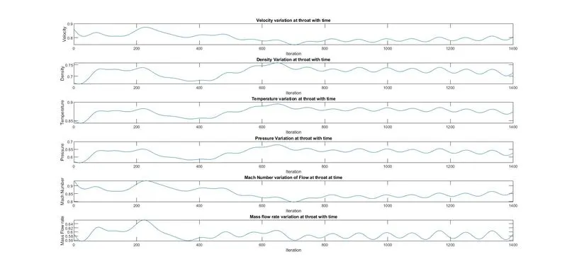
The following plots are plotted for throat section
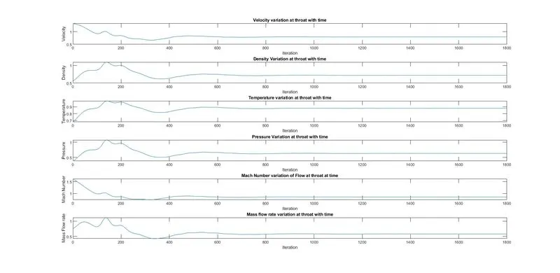
From above graphs, it is observed tht after 1000 iterations or t=0.01*1000=10 sec, the profiles are same.
** Code for conservative method
clear all
close all
clc

%% Create 1D domain
n=31;
L=3;
x=linspace(0,L,n);
dx=x(2)-x(1);
th=(n-1)/2;       % Location of throat
%% Constants
gama=1.4;

%% Time steps
nt=1400;
dt=0.01;

%% initial values of properties
for q=1:n
    if x(q)<=0.5
        rho(q)=1;
        t(q)=1;
    end
    if x(q)>0.5 && x(q)<=1.5
        rho(q)=1-0.366*(x(q)-0.5);
        t(q)=1-0.167*(x(q)-0.5);
    end
    if x(q)>1.5
        rho(q)=0.634-0.3867*(x(q)-1.5);
        t(q)=0.833-0.3507*(x(q)-1.5);
    end
end
% Area
a=1+2.2*(x-1.5).^2;
% Velocity
v=0.59./(rho.*a);

%% Source terms
u1=rho.*a;
u2=rho.*a.*v;
u3=rho.*(t./(gama-1)+(gama/2)*v.^2).*a;


%% CFL number
cfl=max((v+sqrt(t))*dt/dx); %Max-CFL is an input to find timestep!

%% Loop counter
iteration=0;
%% Loops
for k=1:nt   % Time loops
    %% Storing old values

    u1_old=u1;
    u2_old=u2;
    u3_old=u3;

    f1=u2;
    %f2=(u2.^2./u1) +(gama/(gama-1))*u3.*((gama-1)*((u3./u2) - (gama/2)*(u2./u1).^2)); Formula mistake
    f2=(u2.^2./u1) +((gama-1)/gama)*(u3 - (gama/2)*(u2.^2./u1));
    f3=gama*(u2.*u3./u1)-((gama*(gama-1)/2)*(u2.^3./u1.^2));


    % Predictor step
    for j=2:n-1
        j2=(1/gama)*rho(j)*t(j)*((a(j+1)-a(j))/dx);
        % Continuity Equation
        du1dt_p(j)=-(f1(j+1)-f1(j))/dx;

        % Momentum Equation
        du2dt_p(j)=-(f2(j+1)-f2(j))/dx + j2;

        % Energy Equation
        du3dt_p(j)=-(f3(j+1)-f3(j))/dx;

        % Solution update
        u1(j)=u1(j)+du1dt_p(j)*dt;
        u2(j)=u2(j)+du2dt_p(j)*dt;
        u3(j)=u3(j)+du3dt_p(j)*dt;
    end

    % Updating premitive variables
    rho=u1./a;
    t=(gama-1)*((u3./u1)-(gama/2)*(u2./u1).^2);

    f1=u2;
    %f2=(u2.^2./u1) +(gama/(gama-1))*u3.*((gama-1)*((u3./u2) - (gama/2)*(u2./u1).^2)); Formula mistake
    f2=(u2.^2./u1) +((gama-1)/gama)*(u3 - (gama/2)*(u2.^2./u1));
    f3=gama*(u2.*u3./u1)-((gama*(gama-1)/2)*(u2.^3./u1.^2));


    % Corrector step
    for j=2:n-1
        j2=(1/gama)*rho(j)*t(j)*((a(j)-a(j-1))/dx);
        % Continuity Equation
        du1dt_c(j)=-(f1(j)-f1(j-1))/dx;

        % Momentum Equation
        du2dt_c(j)=-(f2(j)-f2(j-1))/dx + j2;

        % Energy Equation
        du3dt_c(j)=-((f3(j)-f3(j-1))/dx);
    end

    % Average
    du1dt=0.5*(du1dt_p+du1dt_c);
    du2dt=0.5*(du2dt_p+du2dt_c);
    du3dt=0.5*(du3dt_p+du3dt_c);

    %% Final Solution updating
    for m=2:n-1
        u1(m)=u1_old(m)+du1dt(m)*dt;
        u2(m)=u2_old(m)+du2dt(m)*dt;
        u3(m)=u3_old(m)+du3dt(m)*dt;
    end

    % Updating premitive / corrector update
    rho=u1./a;
    t=(gama-1)*((u3./u1)-(gama/2)*(u2./u1).^2);
    v=u2./u1;

    %% Apply boundary condition
    % Inlet:
    u1(1)=a(1);
    u2(1)=2*u2(2)-u2(3);
    v(1) = u2(1)/u1(1); % write v(1) using updated u1(1) and u2(1)
    u3(1)=u1(1)*(t(1)/(gama-1)+(gama/2)*(v(1).^2));

    % Outlet:
    u1(n)=2*u1(n-1)-u1(n-2);
    u2(n)=2*u2(n-1)-u2(n-2);
    u3(n)=2*u3(n-1)-u3(n-2);


    iteration=iteration+1;
    % Pressure
    p=rho.*t;
    % MACH NUMBER
    mach=v./sqrt(t);
    % Mass Flow rate
    m=rho.*a.*v;


    %% Storing values at throat
    rho_th(k)=rho(th);       % Density at throat
    v_th(k)=v(th);           % Velocity at throat
    t_th(k)=t(th);           % Temperature at throat
    p_th(k)=p(th);           % Pressure at throat
    mach_th(k)=mach(th);     % Mach number at throat
    m_th(k)=m(th);           % Mass flow rate at throat

    %% Time wise variation plots
    % Mass flow rate
    figure(1)
    hold on
    if k==1
        plot(x,m)
        xlabel('Nozzle Length')
        ylabel('mass flow rate')
    end
    if k==250
        plot(x,m)
        xlabel('Nozzle Length')
        ylabel('mass flow rate')
    end
    if k==500
        plot(x,m)
        xlabel('Nozzle Length')
        ylabel('mass flow rate')
    end
    if k==750
        plot(x,m)
        xlabel('Nozzle Length')
        ylabel('mass flow rate')
    end
    if k==1000
        plot(x,m)
        xlabel('Nozzle Length')
        ylabel('mass flow rate')
    end
    if k==1200
        plot(x,m)
        xlabel('Nozzle Length')
        ylabel('mass flow rate')
    end
    if k==1400
        plot(x,m)
        xlabel('Nozzle Length')
        ylabel('mass flow rate')
    end
    legend('t=0.01','t=2.5','t=5','t=7.5','t=10','t=15','t=18')

    figure(3)
    hold on
    if k==1
        plot(x,mach)
        xlabel('Nozzle Length')
        ylabel('mach number')
    end
    if k==250
        plot(x,mach)
        xlabel('Nozzle Length')
        ylabel('mach number')
    end
    if k==500
        plot(x,mach)
        xlabel('Nozzle Length')
        ylabel('mach number')
    end
    if k==750
        plot(x,mach)
        xlabel('Nozzle Length')
        ylabel('mach number')
    end
    if k==1000
        plot(x,mach)
        xlabel('Nozzle Length')
        ylabel('mach number')
    end
    if k==1200
        plot(x,mach)
        xlabel('Nozzle Length')
        ylabel('mach number')
    end
    if k==1400
        plot(x,mach)
        xlabel('Nozzle Length')
        ylabel('mach number')
    end
    legend('t=0.01','t=2.5','t=5','t=7.5','t=10','t=12','t=14')

    figure(4)
    hold on
    if k==1
        plot(x,p)
        xlabel('Nozzle Length')
        ylabel('pressure')
    end
    if k==250
        plot(x,p)
        xlabel('Nozzle Length')
        ylabel('pressure')
    end
    if k==500
        plot(x,p)
        xlabel('Nozzle Length')
        ylabel('pressure')
    end
    if k==750
        plot(x,p)
        xlabel('Nozzle Length')
        ylabel('pressure')
    end
    if k==1000
        plot(x,p)
        xlabel('Nozzle Length')
        ylabel('pressure')
    end
    if k==1200
        plot(x,p)
        xlabel('Nozzle Length')
        ylabel('pressure')
    end
    if k==1400
        plot(x,p)
        xlabel('Nozzle Length')
        ylabel('pressure')
    end
    legend('t=0.01','t=2.5','t=5','t=7.5','t=10','t=12','t=14')

    figure(2)
    hold on
    if k==1
        plot(x,v)
        xlabel('Nozzle Length')
        ylabel('velcity')
    end
    if k==250
        plot(x,v)
        xlabel('Nozzle Length')
        ylabel('velcity')
    end
    if k==500
        plot(x,v)
        xlabel('Nozzle Length')
        ylabel('velcity')
    end
    if k==750
        plot(x,v)
        xlabel('Nozzle Length')
        ylabel('velcity')
    end
    if k==1000
        plot(x,v)
        xlabel('Nozzle Length')
        ylabel('velcity')
    end
    if k==1200
        plot(x,v)
        xlabel('Nozzle Length')
        ylabel('velcity')
    end
    if k==1400
        plot(x,v)
        xlabel('Nozzle Length')
        ylabel('velcity')
    end
    legend('t=0.01','t=2.5','t=5','t=7.5','t=10','t=12','t=14')


end

%% Plotting
figure(3)
plot(x,v,'color','r')
title(sprintf('Iteration=%d',iteration))
xlabel('Nozzle Length')
ylabel('Velocity')
grid on


figure(4)
plot(x,m,'color','g','linewidth',2)
xlabel('Nozzle Length')
ylabel('Mass Flow Rate')
title(sprintf('Iteration=%d',iteration))

figure(5)
plot(x,rho,'color','b')
title(sprintf('Iteration=%d',iteration))
xlabel('Nozzle Length')
ylabel('Density')
grid on


figure(6)
plot(x,t,'color','g')
title(sprintf('Iteration=%d',iteration))
xlabel('Nozzle Length')
ylabel('Temperature')
grid on

figure(7)
subplot(6,1,1)
plot(v_th)
xlabel('Iteration')
ylabel('Velocity')
title('Velocity variation at throat with time')

subplot(6,1,2)
plot(rho_th)
xlabel('Iteration')
ylabel('Density')
title('Density Variation at throat with time')

subplot(6,1,3)
plot(t_th)
xlabel('Iteration')
ylabel('Temperature')
title('Temperature variation at throat with time')

subplot(6,1,4)
plot(p_th)
xlabel('Iteration')
ylabel('Pressure')
title('Pressure Variation at throat with time')

subplot(6,1,5)
plot(mach_th)
xlabel('Iteration')
ylabel('Mach Number')
title('Mach Number variation of Flow at throat at time')

subplot(6,1,6)
plot(m_th)
xlabel('Iteration')
ylabel('Mass Flow rate')
title('Mass flow rate variation at throat with time')
# Results
A. Steady
1. Velocity
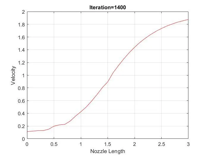
Velocity is increasing. This shows that flow is accelerated. This plot is nearly similar to non conservative method plot.
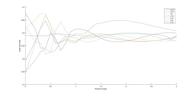
2. mass flow rate
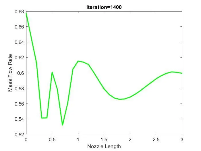
Mass flow rate is also showing variations. This plot is not similar to non conservative method plot. The wiggles are observed in the converging part.
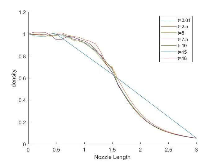
3. Density
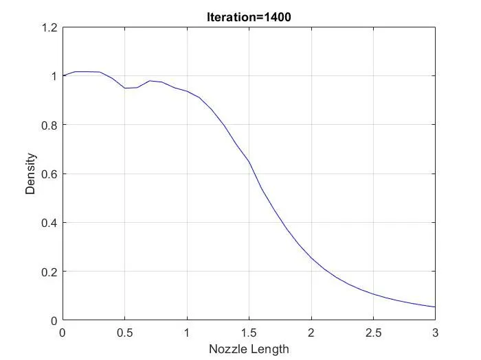
Density is reducing from inlet to outlet. This plot similar to non conservative plot.
4. Temperature
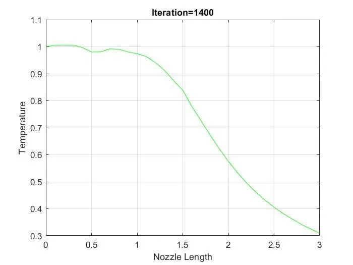
Temperature is reducing from inlet to outlet.
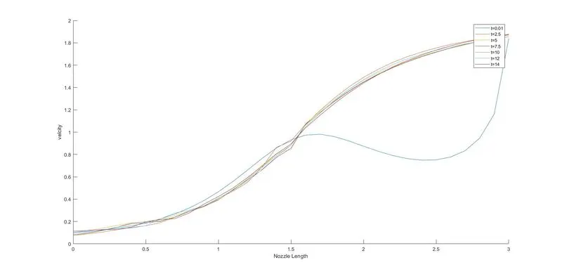
B. Time variation of variation
1. Velocity
2. Mass flow rate
3. Density
4. Temperature
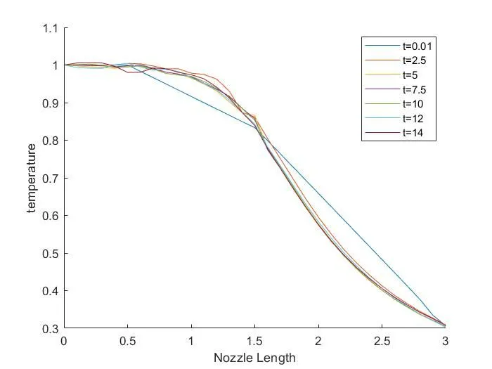
Comment: From all plots, it is seen that steady state is reached sfter t=10 sec.
C. Variation of variables inside nozzle
** Normalized mass flow rate comparision
The figure on LHS is obtained by conservative method while the figure on RHS is obtianed by non conservative method.
We can see that the mass flow rate is minimum at throat on right side figure. But in Left side figure, the mass flow rate is minimum just before throat. The profile is abruptly same.