Week 12 - Validation studies of Symmetry BC vs Wedge BC in OpenFOAM vs Analytical H.P equation

In this challenge you will simulate the same problem as in week 1 but by applying Symmetry Boundary Condition. You will do the simulation for the below mentioned angles using both symmetry and wedge boundary conditions and validate them with HP equations like you did in week 11 challenge.

Angles to test:

• 10
• 25
• 45

Solution:

The major chunk of the theory associated witht the present problem has already been mentioned in the previous assignment. The major solution variables from the haigen poiselli flow are:

V_max_analytical=0.9347'

Entrance Length_analytical=0.504

Delta_p=1.0074

In the blockmesh dict file, P and U file the front and back face are needed to be changed to the type symmetry and then the simulations can be run using the commands stated in the previous assignment.

blockmesh dict:

/*----------------------------------*- C++ -*------------------------------------*\
 ========= | 
 \\ / F ield | OpenFOAM: The Open Source CFD Toolbox 
 \\ / O peration | Website: https://openfoam.org 
 \\ / A nd | Version: 7 
 \\/ M anipulation | 
\*----------------------------------------------------------------------------------*/
FoamFile
{
     version 	 2.0;
      format 	 ascii;
       class 	 dictionary;
      object 	 blockMeshDict;
}
// * * * * * * * * * * * * * * * * * * * * * * * * * * * * * * * * * * * * * //

convertToMeters 1;

vertices
(
	 (0 0 0)
	 (0 1.992389e-03 1.743115e-04)
	 (0 1.992389e-03 -1.743115e-04)
	 (1.204000e+00 0 0)
	 (1.204000e+00 1.992389e-03 1.743115e-04)
	 (1.204000e+00 1.992389e-03 -1.743115e-04)
);

blocks
(
	 hex (0 3 5 2 0 3 4 1) (300 30 1) SimpleGrading (1 0.1 1)

);

edges
(
	 arc 1 2 (0 2.000000e-03 0)
	 arc 4 5 (1.204000e+00 2.000000e-03 0)
);

boundary
(
	 inlet 
	 {
		 type patch;
		 faces
		 (
			 (0 1 2 0)
		 );
	 }
	 outlet
	 {
		 type patch;
		 faces
		 (
			 (3 5 4 3)
		 );
	 }
	 top
	 {
		 type wall;
		 faces
		 (
			 (1 4 5 2)
		 );
	 }
	 front
	 {
		 type symmetry;
		 faces
		 (
			 (0 3 4 1)
		 );
	 }
	 back
	 {
		 type symmetry;
		 faces
		 (
			 (0 2 5 3)
		 );
	 }
	 axis
	 {
		 type empty;
		 faces
		 (
			 (0 3 3 0)
		 );
	 }
); 

mergePatchPairs
(
);
// * * * * * * * * * * * * * * * * * * * * * * * * * * * * * * * * * * * * * //

P file:

/*--------------------------------*- C++ -*----------------------------------*\
  =========                 |
  \\      /  F ield         | OpenFOAM: The Open Source CFD Toolbox
   \\    /   O peration     | Website:  https://openfoam.org
    \\  /    A nd           | Version:  9
     \\/     M anipulation  |
\*---------------------------------------------------------------------------*/
FoamFile
{
    format      ascii;
    class       volScalarField;
    location    "0";
    object      p;
}
// * * * * * * * * * * * * * * * * * * * * * * * * * * * * * * * * * * * * * //

dimensions      [0 2 -2 0 0 0 0];

internalField   uniform 0;

boundaryField
{
 inlet
 {
 type zeroGradient;
 }
 outlet
 {
 type fixedValue;
 value uniform 1.0073;
 }
 axis
 {
 type empty;
 }
 top
 {
 type zeroGradient;
 }
 front
 {
 type symmetry;
 }
 back
 {
 type symmetry;
 }
}
// ************************************************************************* //

U file:

/*--------------------------------*- C++ -*----------------------------------*\
  =========                 |
  \\      /  F ield         | OpenFOAM: The Open Source CFD Toolbox
   \\    /   O peration     | Website:  https://openfoam.org
    \\  /    A nd           | Version:  9
     \\/     M anipulation  |
\*---------------------------------------------------------------------------*/
FoamFile
{
    format      ascii;
    class       volVectorField;
    location    "0";
    object      U;
}
// * * * * * * * * * * * * * * * * * * * * * * * * * * * * * * * * * * * * * //

dimensions      [0 1 -1 0 0 0 0];

internalField   uniform (1 0 0);

boundaryField
{
 inlet
 {
 type fixedValue;
 value uniform (0.4686 0 0);
 }
 outlet
 {
 type zeroGradient;
 }
 axis
 {
 type empty;
 }
 top
 {
 type fixedValue;
 value uniform (0 0 0);
 }
 front
 {
 type symmetry;
 }
 back
 {
 type symmetry;
 }
}
// ************************************************************************* //

Validate Hydro-dynamic length with the numerical result.

Wedge case:

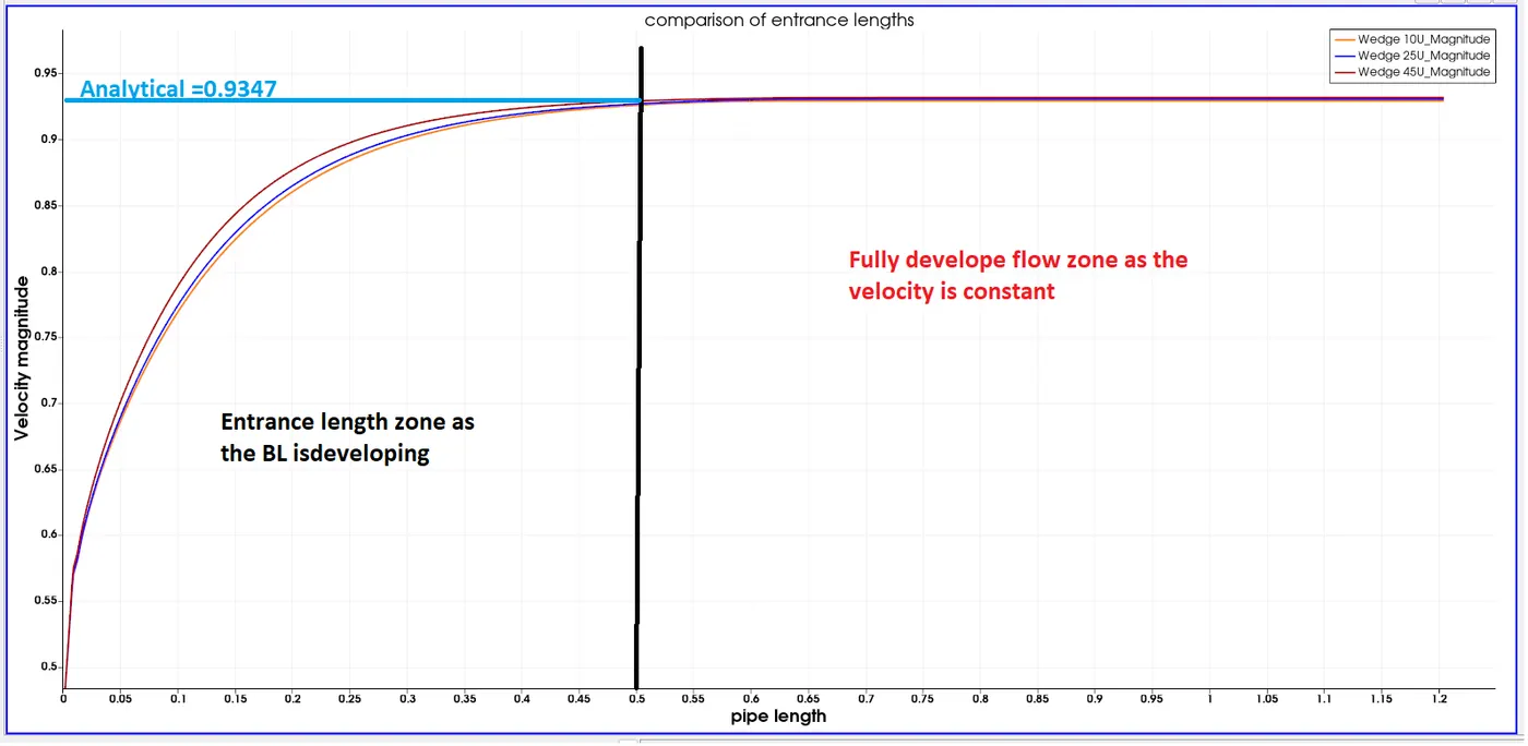
It can be observed that the velocity reaches an maximum value after the fluid passes a distance of 0.5m which is the analytical entrance length.

Symmetry Case:

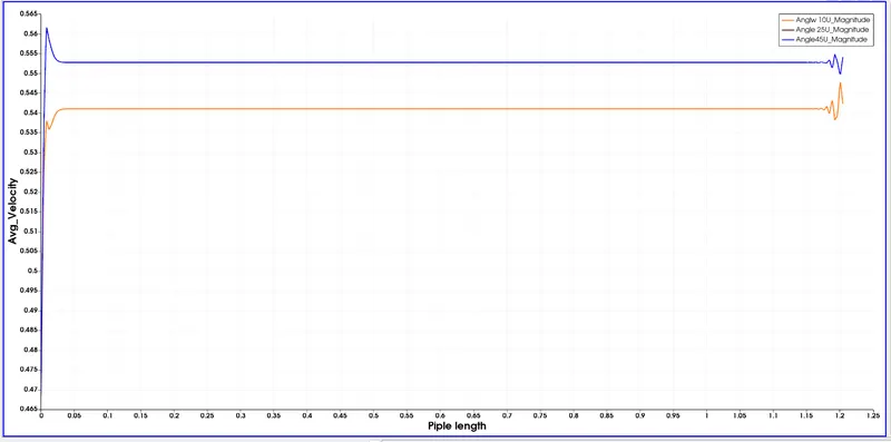
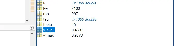
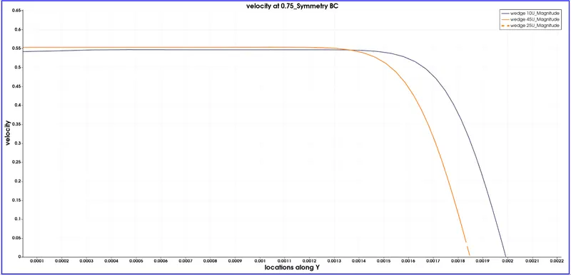
The velocity profile looks quiet unrealistic by the velocity indicated here is the average velocity at the centre of the pipe, which is around 0.467 Analytical value.

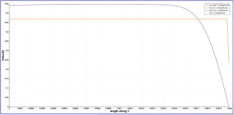
Velocity profile at various locations along the length of the pipe is shown in the above figure and it amtches with the analytical behaviour of the flow through the pipe.

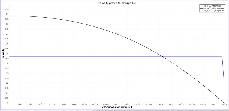
This is the velocity profile in case of the wedge boundary condition at wedge angle1o and for the various locations along the length of the pipe

The shear stress distribution analytically is shown below:

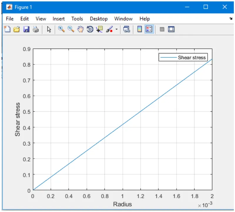
The shear stress increases from the centre of the pipe to the wall as the velocity gradient is high near the wall due to the no slip boundary condition

In order to plot the shear stress at a location i.e. X=0.7 we need to store the values as excel from the paraview and the excel values can be imported to matlab. The following code is written in matlab to make the plot of the shear stress

Function file

function [tau_cfd] = TAU(R, v_cfd)
mu = 0.89e-3;

dR = R(2)-R(1);

for i = 1:length(R)-1
 du = v_cfd(i+1)-v_cfd(i);
 dU = abs(du);
 tau_cfd(i) = mu*(dU/dR);
end


end

Main File

%% used to post process the data on the 
clear all
clc

% uiopen('G:\assignment\Week10\velocity_analyticak.csv',1)
% velocityanalyticak=xlsread('velocity_analyticak.csv');
% arc_length=velocityanalyticak(:,2);
R_Sym=0.002;
L=1.2040;
mu = 0.89e-3;

load('data.mat')

%%%%%%%%%%%%%%%%%%%%%%%%%%%%%%%%%%%%%%%%%%%%%
%% SHear for wedge
R_Sym = Symmetry(:,1);
[Symmetry_10] = TAU(R_Sym,Symmetry(:,2));
[Symmetry_25] = TAU(R_Sym,Symmetry(:,3));
[Symmetry_45] = TAU(R_Sym,Symmetry(:,4));

R_Del = wedge(:,1);

[wedge_10] = TAU(R_Del,wedge(:,2));
[wedge_25] = TAU(R_Del,wedge(:,3));
[wedge_45] = TAU(R_Del,wedge(:,4));


figure(1)
plot(R_Sym(2:end), Symmetry_10, 'r', 'LineWidth', 2)
hold on
grid on
plot(R_Sym(2:end), Symmetry_25, 'b','LineWidth', 2)
hold on 
plot(R_Sym(2:end), Symmetry_45, 'm','LineWidth', 2)
xlabel('location in Ydirection')
ylabel('shear stress')
legend('Angle_{10}', 'Angle_{25}', 'Angle_{45}')
title('Symmetry Boundary condition')
hold off

figure(2)
plot(R_Del(2:end), wedge_10, 'r', 'LineWidth', 2)
hold on 
grid on 
plot(R_Del(2:end), wedge_25, 'b','LineWidth', 2)
hold on 
plot(R_Del(2:end), wedge_45, 'm','LineWidth', 2)
xlabel('location in Ydirection')
ylabel('shear stress')
legend('Angle_{10}', 'Angle_{25}', 'Angle_{45}')
title('Wedge Boundary condition')

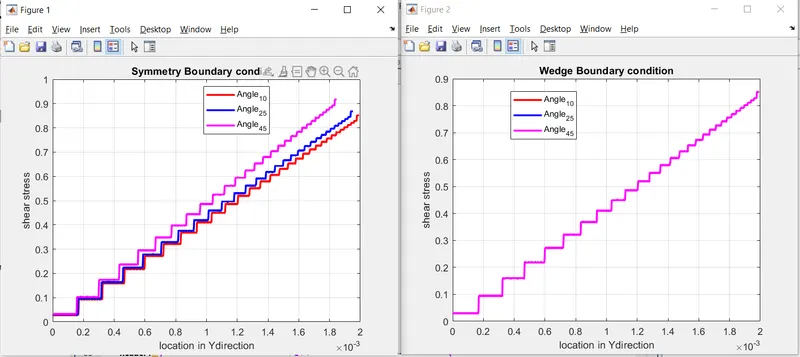
From the plot it can be ibserved that, the shear stress distribution follows the trend but

In wedge boundary condition: The values are close to the analytical and the shear stress distribution is same for all the three wedge angles in the developed zone

In the symmetric bondary condition, it can be observed that as the wedge angle increases the value of the stress is over estimated.

The stair case profile is essentially due to the step variation in the finite volume formulation.

When the Symmetry boundary condition condition are applied the average velocity is seen at the centereline of the pipe