Week 7 - Simulation of a 1D Super-sonic nozzle flow simulation using Macormack Method

Quasi 1D subsonic-supersonic nozzle

Following is a schematic representation of nozzle

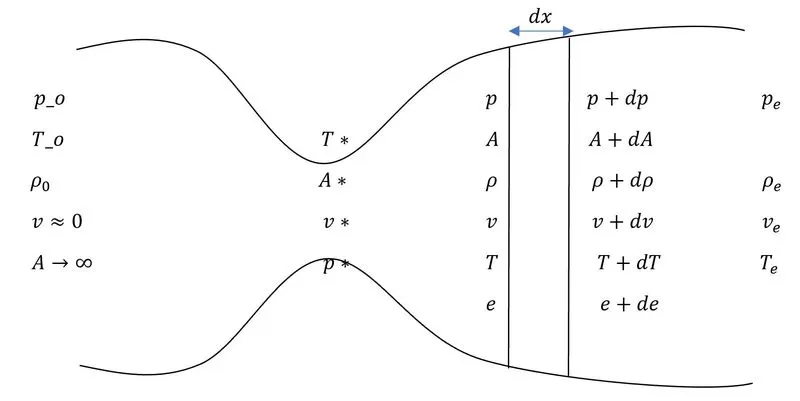
considering an elemental strip we can derive mass, momentum, and energy equations as follows:

Mass conservation for fine control volume:

The integral form of the integral equation is:

`∂/(∂t) ∫_vρdV+ ∫_s ρ \vecV .dA=0`

Let us apply this equation to the control volume drawn above:

The volume integral then can be written (considering the thickness of the element tending to zero) as:

`∂/(∂t) ∫_v ρdV =∂/(∂t)(ρA dx)`

where, `dx` is the thickness of the element. The surface integral can be written with the same philosophy as:

`∫_s ρ \vecV .dA=-ρvA+(p+dp)(v+dv)(A+dA)=ρvdA+ρAdv+Avdρ=d(ρAv)`

where, is the component of velocity in the direction of nozzle flow (i.e., axis)

On clubbing them up we get:

`∂/(∂t) (ρA dx)+d(ρAv)=0`

On dividing both side by we get:

`\frac{∂}{∂t} (ρA)+ \frac{∂}{∂x} (ρAv) =0` (1)

Equation 1 is the continuity equation (mass conservation) in conservative form.

Momentum conservation:

Integral form of the inviscid momentum equation along the nozzle longitudinal direction is:

`∂/(∂t) ∫_v (ρv)dV+ ∫_s (ρv \vecV ). dA=-∫_s(pdA)_x`

In a limit when tend to zero the first term and second terms of LHS can be written as:

`∂/(∂t) ∫_v (ρv)dV=∂/(∂t)(ρvA dx)`

`∫_s (ρv \vecV ) .dA=-ρv^2 A+(ρ+dρ)(v+dv)(A+dA)`

And the RHS can be written as:

`∫_s (pdA)_x =-pA+(p+dp)(A+dA)-2p((dA)/2)`

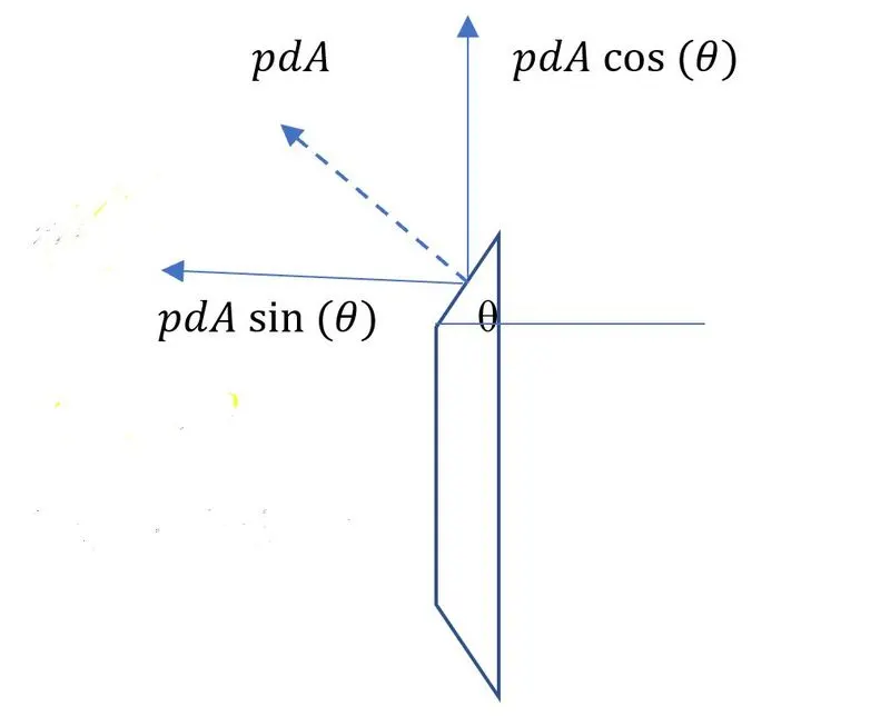
On the inclined area the net projected area will be `2p dA cos(\theta)` (both from top and bottom). As `sin(\theta)=(dA)/(ds)` so, this component will be equal to `2 (pdA)/2` . Where `ds` is the length of inclined surface. The elemental strip is shown below.

On combining them all into the main equation it becomes:

`∂/(∂t) (ρvA dx)-ρv^2 A+(ρ+dρ)(v+dv)(A+dA)=-(-pA+(p+dp)(A+dA)-2p ((dA)/2))`

After slight rearrangement and division by it becomes:

`∂/(∂t) (ρvA)+∂/(∂x) (ρv^2 A)=-A (∂p)/(∂x)` (2)

Now Equation 2 is the conservative form of momentum equation.

On multiplying Eq. 1 by we get:

`v ∂/(∂t) (ρA)+v ∂/(∂x) (ρAv)=0`

It can also be written as:

`∂/(∂t) (ρAv)-ρA (∂v)/(∂t)+∂/(∂x) (ρAv v)-ρAv (∂v)/(∂x)=0`

`∂/(∂t) (ρAv)+∂/(∂x) (ρAv^2 )-ρA (∂v)/(∂t)-ρAv (∂v)/(∂x)=0`

Now replacing the value of LhS from Eq. 2 in the above equation will lead to:

`-A (∂p)/(∂x) -ρA (∂v)/(∂t)-ρAv (∂v)/(∂x)=0`

hence,

`ρ (∂v)/(∂t)+ρv (∂v)/(∂x)=-(∂p)/(∂x)` (3)

Eq. 3 is the momentum equation in nonconservative form.

Energy conservation:

Integral form of the inviscid momentum equation along the nozzle longitudinal direction is:

`∂/(∂t) ∫_v ρ(e+v^2/2)dV+ ∫_s ρ(e+v^2/2) \vecV . dA=-∫_s p \vecV . dA`

In a limit when tend to zero the first term and second terms of LHS can be written as:

`∂/(∂t) ∫_v ρ(e+v^2/2)dV=∂/(∂t) (ρ(e+v^2/2)A dx)`

`∫_sp \vecV dA= (-pvA+(p+dp)(A+dA)(v+dv)-2pv((dA)/2))`

On slight rearrangement above equation becomes:

`∂/(∂t) (ρ(e+v^2/2)A)+∂/(∂x) (ρ(e+v^2/2)vA)=-∂/(∂x)(pAv)` (4)

Eq. 4. is the energy equation in conservative form expressed in `e+v^2/2` .

On multiplying Eq. 2 by `v` we get:

`∂/(∂t) (ρ v^2/2 A)+∂/(∂x) (ρ v^2/2 Av)=-Av (∂p)/(∂x)`

On subtracting above equation from Eq. 4 we get:

`∂/(∂t) (ρ(e+v^2/2-v^2/2)A)+∂/(∂x) (ρ(e+v^2/2-v^2/2)vA)=-p ∂/(∂x)(Av)`

`∂/(∂t) (ρeA)+∂/(∂x) (ρevA)=-p ∂/(∂x)(Av)` (5)

Eq. 5. is the energy equation in conservative form expressed in (`e`).

If we multiply Eq. 1 by `e` and subtract it from Eq. 5 we will get:

`ρA ∂/(∂t) (e)+ρvA ∂/(∂x) (e)=-p ∂/(∂x)(Av)`

On expanding RHS and dividing the equation by `A` will result in:

`ρ ∂/(∂t) (e)+ρv ∂/(∂x) (e)=-p ∂/(∂x)(v)-pv ∂/(∂x)(ln⁡A)` (6)

Eq. 6 is the energy equation in nonconservative form expressed in (`e`).

On replacing the value of internal energy (`e`) as `c_vT` we will get:

`ρc_v (∂T)/(∂t)+ρvc_v (∂T)/(∂x)=-p (∂v)/(∂x)-pv ∂/(∂x)(ln⁡A)` (7)

Eq. 7 is the energy equation in nonconservative form expressed in (`T`).

Law	Conservative	Nonconservative
Conservation of mass	`∂/(∂t) (ρA)+∂/(∂x) (ρAv)=0`	`∂/(∂t) (ρA)+ρA ∂/(∂x) (v)+ρv ∂/(∂x) (A)+vA ∂/(∂x) ρ)=0`
Conservation of momentum	`∂/(∂t) (ρvA)+∂/(∂x) (ρv^2 A)=-A (∂p)/(∂x)`	`ρ (∂v)/(∂t)+ρv (∂v)/(∂x)=-(∂p)/(∂x)`
Conservation of energy	`∂/(∂t) (ρ(e+v^2/2)A)+∂/(∂x) (ρ(e+v^2/2)vA)=-∂/(∂x)(pAv)` `∂/(∂t) (ρeA)+∂/(∂x) (ρevA)=-p ∂/(∂x)(Av)`	`ρ ∂/(∂t) (e)+ρv ∂/(∂x) (e)=-p ∂/(∂x)(v)-pv ∂/(∂x)(ln⁡A)` `ρc_v (∂T)/(∂t)+ρvc_v (∂T)/(∂x)=-p (∂v)/(∂x)-pv ∂/(∂x)(ln⁡A)`

Above table shows that we have 3 equation and 4 unknowns (`p,v,T, \rho`), so one more equation is required which will come from equation of state i.e., `p=\rho R T` . On differentiating 'p' and substituting it into momentum and energy equations we will get 3 equation and 3 unknowns as:

Dimensional form of nonconservative equations
Conservation of mass	`∂/(∂t) (ρA)+ρA ∂/(∂x) (v)+ρv ∂/(∂x) (A)+vA ∂/(∂x) (ρ)=0`
Conservation of momentum	`ρ (∂v)/(∂t)+ρv (∂v)/(∂x)=-R(ρ (∂T)/(∂x)+ T (∂ρ)/(∂x))`
Conservation of energy	`c_v (∂T)/(∂t)+ρvc_v (∂T)/(∂x)=-ρRT((∂v)/(∂x)+v ∂/(∂x) (ln⁡A ))`

Non-dimensional form of nonconservative equations
Conservation of mass	`∂/(∂t') (ρ')+ρ'∂/(∂x^' ) (v^' )+ρ'v'∂/(∂x')( ln⁡ A^' )+v'∂/(∂x') (ρ')=0`
Conservation of momentum	`(∂v^')/(∂t^' )+v'(∂v^')/(∂x^' )=-1/γ ((∂T')/(∂x')+(T')/(ρ') (∂ρ')/(∂x'))`
Conservation of energy	`(∂T')/(∂t')+v (∂T')/(∂x')=-(γ-1)T'((∂v')/(∂x')+v'∂/(∂x) (ln⁡A' ))`

The non-dimensionalization has been done considering:

`x^'=x/l ; ρ^'=ρ/ρ_0 ; T^'=T/T_0 ; v^'=v/a_0 ; t^'=t/(l/a_0 ) ;A^'=A/A^{\star}`

where `a_0=√(γRT_0)`

Finite difference discretization (Nonconservative form)

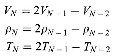
For this we have adopted nondimensional version of conservations equations but for the sake of simplicity the primed variables are replaced by unprimed.

As the equation is hyperbolic in nature so time marching approach has been adopted. Maccormack’s algorithm is used to solve this time marching problem. This is a predictor-corrector technique. In the predictor step the space derivatives are discretized using forward difference whereas, in the corrector step they are discretized using backward difference.

Predictor step
(1) Obtaining predictor slopes
Conservation of mass	`∂/(∂t) (ρ)=-ρ ∂/(∂x) (v)-ρv ∂/(∂x)( ln⁡A )-v ∂/(∂x) (ρ)` `((∂ρ)/(∂t))_p^t=(-ρ_i ((v_(i+1)-v_i ))/(Δx)-ρ_i v_i ((ln⁡(A)_(i+1)-ln⁡(A)_i ))/(Δx)-v_i ((ρ_(i+1)-ρ_i ))/(Δx))^t`
Conservation of momentum	`(∂v)/(∂t)=-v (∂v)/(∂x)-1/γ ((∂T)/(∂x)+T/ρ (∂ρ)/(∂x))` `((∂v)/(∂t))_p^t=(-v_i ((v_(i+1)-v_i ))/(Δx)-1/γ (((T_(i+1)-T_i ))/(Δx)+T_i/ρ_i ((ρ_(i+1)-ρ_i ))/(Δx)))^t`
Conservation of energy	`(∂T)/(∂t)=-v (∂T)/(∂x)-(γ-1)T((∂v)/(∂x)+v ∂/(∂x) (ln⁡A ))` `((∂T)/(∂t))_p^t=(-v_i ((T_(i+1)-T_i ))/(Δx)-(γ-1) T_i (v_i ((ln⁡(A)_(i+1)-ln⁡(A)_i ))/(Δx)+((v_(i+1)-v_i ))/(Δx)))^t`
(2) Obtaining the values of v, `rho` , and T based on above predicted time derivatives for time step `t+\Delta t`
`ρ_i=ρ_(old,i)^t+((∂ρ)/(∂t))_p^t Δt` `v=v_(old,i)^t+((∂v)/(∂t))_p^t Δv` `T_i=T_(old,i)^t+((∂T)/(∂t))_p^t ΔT`

Corrector step
(1) Obtaining corrector slope based on above evaluated values of v, , and T for the time step
Conservation of mass	`((∂ρ)/(∂t))_c^(t+Δt)=(-ρ_i ((v_i-v_(i-1) ))/(Δx)-ρ_i v_i ((ln⁡(A)_i-ln⁡(A)_(i-1) ))/(Δx)-v_i ((ρ_i-ρ_(i-1) ))/(Δx))^(t+Δt)`
Conservation of momentum	`((∂v)/(∂t))_c^(t+Δt)=(-v_i ((v_i-v_(i-1) ))/(Δx)-1/γ (((T_i-T_(i-1) ))/(Δx)+T_i/ρ_i ((ρ_i-ρ_(i-1) ))/(Δx)))^(t+Δt)`
Conservation of energy	`((∂T)/(∂t))_c^(t+Δt)=(-v_i ((T_i-T_(i-1) ))/(Δx)-(γ-1) T_i (v_i ((ln⁡(A)_i-ln⁡(A)_(i-1) ))/(Δx)+((v_i-v_(i-1) ))/(Δx)))^(t+Δt)`
(2) Based on predictor and corrector slope an average slope is evaluated
`((∂ρ)/(∂t))_(avj)=1/2 (((∂ρ)/(∂t))_p^t+((∂ρ)/(∂t))_c^(t+Δt) )` `((∂v)/(∂t))_(avj)=1/2 (((∂v)/(∂t))_p^t+((∂v)/(∂t))_c^(t+Δt) )` `((∂T)/(∂t))_(avj)=1/2 (((∂T)/(∂t))_p^t+((∂T)/(∂t))_c^(t+Δt) )`
(3) Finally the of v, , and T at time step is obtained as:
`ρ_i^(t+Δt)=ρ_(old,i)^t+((∂ρ)/(∂t))_(avj) Δt` `v_i^(t+Δt)=v_(old,i)^t+((∂v)/(∂t))_(avj) Δt` `T_i^(t+Δt)=T_(old,i)^t+((∂T)/(∂t))_(avj) Δt`

Time step calculations:

first `\Delta t ` is evaluated at each node by following equaiton and then minimum of all the value is taken as time step.

`\Deltat_i=0.5dx/(sqrt(T_(i))+v_(i))`

where 0.5 is the value of Courent number taken.

Boundary conditions:

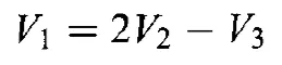
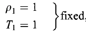
inlet:

outlet:

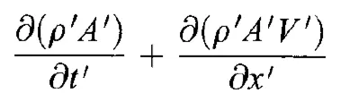
Finite difference discretization (Conservative form)

Mass conservation:

Momentum conservation:

Energy conservation:

Let:

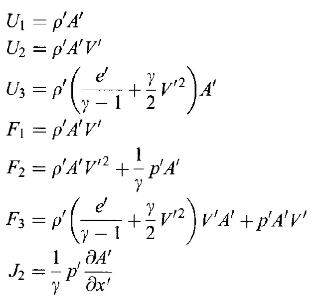
where U, F, and J are solution vector, flux vectro, and source term.

Now we have to solve following equations:

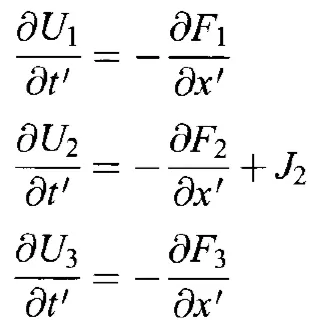
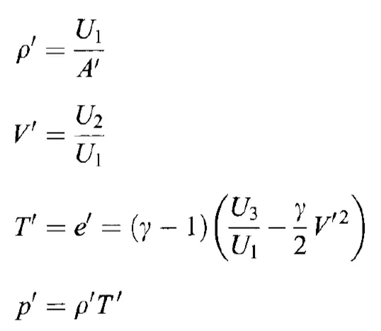
The value of flux terms should not be evaluated based on premitive variables insted it should be done on the basis of `U_1`, `U_2` and `U_3` as follows:

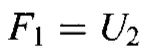
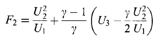
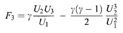
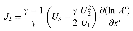
where,

Boundary conditions:

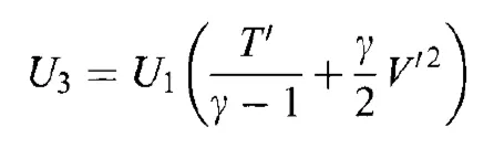
inlet:

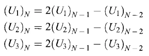
exit:

Code and resutls

Nozzle profile:

`A=1+2.2(x-1.5)^2`

Initial conditions nonconservative form:

`ρ=1-0.3146x`
`T=1-0.2314x`
`v=(0.1+1.09x)T^(1/2)`

Initial conditions for conservative form:

(x(i)>=0 && x(i)<=0.5)
rho(i)=1.0;
T(i)=1.0;

(x(i)>=0.5 && x(i)<=1.5)
rho(i)=1-0.366*(x(i)-0.5);
T(i)=1-0.167*(x(i)-0.5);

(x(i)>=1.5 && x(i)<=3.5)
rho(i)=0.634-0.3879*(x(i)-1.5);
T(i)=0.833-0.3507*(x(i)-1.5);

v=0.59./(rho.*A);

Matlab function for non-conservative form:

function [p,rho,T,v,Ma,m_dot,x,A,dx]=non_conservative_app(L,gama,n,Ts)


%######################################
%            Grid generation
%######################################
x=linspace(0,L,n);
dx=L/(n-1);
%--------------------
% Nozzle Area
%--------------------
A=1+2.2*(x-1.5).^2;

% Intermediate time step
dt_i=zeros(1,n);

%######################################
%            Initial Conditions
%######################################

rho=1-0.3146*x;
T=1-0.2314*x;
v=(0.1+1.09*x).*T.^(1/2);

rho_old=rho;
T_old=T;
v_old=v;

%######################################
%              Time Marching
%######################################
for t = 1:Ts
%######################################
%              Predictor Step
%######################################
    drho_dt_p=zeros(1,n);
    dv_dt_p=zeros(1,n);
    dT_dt_p=zeros(1,n);


    for i = 2:n-1
        CE1=rho(i)*(v(i+1)-v(i))/dx;
        CE2=rho(i)*v(i)*(log(A(i+1))-log(A(i)))/dx;
        CE3=v(i)*(rho(i+1)-rho(i))/dx;
        drho_dt_p(i)=-CE1-CE2-CE3;
       %-----------------------

        ME1=v(i)*(v(i+1)-v(i))/dx;
        ME2=((T(i+1)-T(i))/dx+(T(i)/rho(i))*(rho(i+1)-rho(i))/dx)/gama;
        dv_dt_p(i)=-ME1-ME2;
       %-----------------------

        EE1=v(i)*(T(i+1)-T(i))/dx;
        EE2=(gama-1)*T(i)*((v(i+1)-v(i))/dx+v(i)*(log(A(i+1))-log(A(i)))/dx);
        dT_dt_p(i)=-EE1-EE2;
        %-----------------------
    end

    %######################################    
    % Time step calculations
    %######################################
    for i = 1:n
        dt_i(i)=0.5*dx/(sqrt(T_old(i))+v_old(i));
    end
    % selecting minimum value    
    dt=min(dt_i);
    dt=round(dt,4);


    %   updated values of ρ,v, and T
    for i = 2:n-1
        rho(i)=rho_old(i)+drho_dt_p(i)*dt;
        v(i)=v_old(i)+dv_dt_p(i)*dt;
        T(i)=T_old(i)+dT_dt_p(i)*dt;
    end 
    %######################################
    %              Corrector Step
    %######################################
    drho_dt_c=zeros(1,n);
    dv_dt_c=zeros(1,n);
    dT_dt_c=zeros(1,n);

    drho_dt_avj=zeros(1,n);
    dv_dt_avj=zeros(1,n);
    dT_dt_avj=zeros(1,n);

    for i = 2:n-1
        CE1=rho(i)*(v(i)-v(i-1))/dx;
        CE2=rho(i)*v(i)*(log(A(i))-log(A(i-1)))/dx;
        CE3=v(i)*(rho(i)-rho(i-1))/dx;
        drho_dt_c(i)=-CE1-CE2-CE3;
    
       %-----------------------

        ME1=v(i)*(v(i)-v(i-1))/dx;
        ME2=((T(i)-T(i-1))/dx+(T(i)/rho(i))*(rho(i)-rho(i-1))/dx)/gama;
        dv_dt_c(i)=-ME1-ME2;
       %-----------------------

        EE1=v(i)*(T(i)-T(i-1))/dx;
        EE2=(gama-1)*T(i)*((v(i)-v(i-1))/dx+v(i)*(log(A(i))-log(A(i-1)))/dx);
        dT_dt_c(i)=-EE1-EE2;
        %-----------------------

       % computing average value of time derivatives
        drho_dt_avj(i)=0.5*(drho_dt_p(i)+drho_dt_c(i));
        dv_dt_avj(i)=0.5*(dv_dt_p(i)+dv_dt_c(i));
        dT_dt_avj(i)=0.5*(dT_dt_p(i)+dT_dt_c(i));
        %-------------------------------------------

        % Final value of parameters at n+1th time step
        rho(i)=rho_old(i)+drho_dt_avj(i)*dt;
        v(i)=v_old(i)+dv_dt_avj(i)*dt;
        T(i)=T_old(i)+dT_dt_avj(i)*dt;
    end
    %##########################################
    %    Boundary Conditions update
    %##########################################
    % updating inlet velocity boundary condition 
    v(1)=2*v(2)-v(3);
    
    % Updating exit boundary conditions
    v(end)=2*v(end-1)-v(end-2);
    rho(end)=2*rho(end-1)-rho(end-2);
    T(end)=2*T(end-1)-T(end-2);
    
    % Pressure evaluation
    p=rho.*T;
    
    % updating the old values by new
    rho_old=rho;
    T_old=T;
    v_old=v;

    % Determination of Mach number
    Ma=v./sqrt(T);
    
    %Mass flow rate calculations
    m_dot=rho.*A.*v;
    
    if mod(t,100)==0
        fprintf('Time step= %d',t);
        fprintf('dt = %f',dt);
    end

    figure(2)
    subplot(4,1,1)
    plot(t,rho(int64(n/2)),'bo',markersize=0.5); 
    hold on
    ylim([0.5,1])
    xlabel('Time')
    ylabel('ρ/ρ_0')
    
    subplot(4,1,2)
    plot(t,T(int64(n/2)),'bo',markersize=0.5)
    hold on
    ylim([0.6,0.95])
    xlabel('Time')
    ylabel('T/T_0')
    
    subplot(4,1,3)
    plot(t,p(int64(n/2)),'bo',markersize=0.5) 
    hold on
    ylim([0.4,0.9])
    xlabel('Time')
    ylabel('p/p_0')
    
    subplot(414)
    plot(t,Ma(int64(n/2)),'bo',markersize=0.5)
    hold on
    ylim([0.8,1.6])
    xlabel('Time')
    ylabel('Ma')

    
     figure(3)
     if (t==1||t==50||t==100||t==150||t==200||t==250 || t==700)
         txt = [num2str(t),'\Deltat'];
         plot(x,m_dot,'-','DisplayName',txt)
         hold on
         xlabel('x')
         ylabel('Non dimensional mass flow')
     end
     legend show    
end
end

Matlab function for conservative form:

function [p,rho,T,v,Ma,m_dot,x,A,dx]=conservative_app(L,gama,n,Ts)

%######################################
%            Grid generation
%######################################
x=linspace(0,L,n);
dx=L/(n-1);
%--------------------
% Nozzle Area
%--------------------
A=1+2.2.*(x-1.5).^2;

%--------------------
%  Initial conditions
%--------------------

rho=zeros(1,n);
T=zeros(1,n);

for i = 1:n
    if (x(i)>=0 && x(i)<=0.5)
        rho(i)=1.0;
        T(i)=1.0;
    elseif (x(i)>=0.5 && x(i)<=1.5)
        rho(i)=1-0.366*(x(i)-0.5);
        T(i)=1-0.167*(x(i)-0.5);
    else
        rho(i)=0.634-0.3879*(x(i)-1.5);
        T(i)=0.833-0.3507*(x(i)-1.5);
    end
end
v=0.59./(rho.*A);

%--------------------
% Solution Vector
%--------------------
u1=rho.*A;
u2=rho.*A.*v;
u3=rho.*(T./(gama-1)+(gama/2).*v.^2).*A;

%-----------------------------------------
% Flux vector in terms of Solution Vector
%-----------------------------------------
f1=u2;
f2=u2.^2./u1+((gama-1)/gama).*(u3-(gama/2).*(u2.^2./u1));
f3=gama*u2.*u3./u1-0.5*gama*(gama-1)*u2.^3./u1.^2;
j2=zeros(1,n);
for i = 2:n-1
    j2(i)=(1/gama)*rho(i).*T(i).*(A(i+1)-A(i))/dx;
end

dt_i=zeros(1,n);  
    
    
u2_old=u2;
u1_old=u1;
u3_old=u3 ;   



%######################################
%              Time Marching
%######################################
for t = 1:Ts

%######################################
%              Predictor Step
%######################################
    du1_dt_p=zeros(1,n);
    du2_dt_p=zeros(1,n);
    du3_dt_p=zeros(1,n);


    for i = 2:n-1
        du1_dt_p(i)=-(f1(i+1)-f1(i))/dx;
       %-----------------------
    
        j2(i)=(1/gama)*rho(i)*T(i)*(A(i+1)-A(i))/dx;
        
        du2_dt_p(i)=-(f2(i+1)-f2(i))/dx+j2(i);
        
       %-----------------------

        du3_dt_p(i)=-(f3(i+1)-f3(i))/dx;
        %-----------------------
    end 

    %######################################    
    % Time step calculations
    %######################################
    for i = 1:n
        dt_i(i)=0.5*dx/(sqrt(T(i))+v(i));
    end

    % selecting minimum value    
    dt=min(dt_i);
    dt=round(dt,4);


    %   updated values of ρ,v, and T
    for i = 2:n-1
        u1(i)=u1_old(i)+du1_dt_p(i)*dt;
        u2(i)=u2_old(i)+du2_dt_p(i)*dt;
        u3(i)=u3_old(i)+du3_dt_p(i)*dt;
    end
    
    %##########################################
    % Evaluation of primitive variables
    %#########################################
    
    rho=u1./A;
    T=(gama-1)*(u3./u1-(gama/2)*u2.^2./u1.^2) ;   
    
    
    %-----------------------------------------
    % Flux vector in terms of Solution Vector
    %-----------------------------------------
    f1=u2;
    f2=u2.^2./u1+((gama-1)/gama)*(u3-(gama/2).*(u2.^2./u1));
    f3=gama*u2.*u3./u1-0.5*gama*(gama-1)*u2.^3./u1.^2;
            
    %######################################
    %              Corrector Step
    %######################################
    du1_dt_c=zeros(1,n);
    du2_dt_c=zeros(1,n);
    du3_dt_c=zeros(1,n);

    du1_dt_avj=zeros(1,n);
    du2_dt_avj=zeros(1,n);
    du3_dt_avj=zeros(1,n);

    for i = 2:n-1
        du1_dt_c(i)=-(f1(i)-f1(i-1))/dx;
       %-----------------------
        
        j2(i)=(1/gama)*rho(i)*T(i)*(A(i)-A(i-1))/dx;
        
        du2_dt_c(i)=-(f2(i)-f2(i-1))/dx+j2(i);
       %-----------------------

        du3_dt_c(i)=-(f3(i)-f3(i-1))/dx;
       %-----------------------

       % computing average value of time derivatives
        du1_dt_avj(i)=0.5*(du1_dt_p(i)+du1_dt_c(i));
        du2_dt_avj(i)=0.5*(du2_dt_p(i)+du2_dt_c(i));
        du3_dt_avj(i)=0.5*(du3_dt_p(i)+du3_dt_c(i));
        %-------------------------------------------

        % Final value of parameters at n+1th time step
        u1(i)=u1_old(i)+du1_dt_avj(i)*dt;
        u2(i)=u2_old(i)+du2_dt_avj(i)*dt;
        u3(i)=u3_old(i)+du3_dt_avj(i)*dt;
    end

    %##########################################
    %    Boundary Conditions update
    %##########################################
    % updating inlet velocity boundary condition 
    u1(1)=A(1)*rho(1);
    u2(1)=2*u2(2)-u2(3);
    v(1)=u2(1)/u1(1);
    u3(1)=u1(1)*(T(1)/(gama-1)+(gama/2)*v(1)^2);
    
    % Updating exit boundary conditions
    u1(end)=2*u1(end-1)-u1(end-2);
    u2(end)=2*u2(end-1)-u2(end-2);
    u3(end)=2*u3(end-1)-u3(end-2);
    
    %##########################################
    %    Evaluation of flux for next time step
    %##########################################
    f1=u2;
    f2=u2.^2./u1+((gama-1)/gama)*(u3-(gama/2)*(u2.^2./u1));
    f3=gama*u2.*u3./u1-0.5*gama*(gama-1)*u2.^3./u1.^2;
    
    %##########################################
    % Evaluation of primitive variables
    %##########################################
    
    rho=u1./A;
    v=u2./u1;
    T=(gama-1)*(u3./u1-(gama/2)*u2.^2./u1.^2);
    p=rho.*T;
    
    %##########################################
    % updating the old values by new
    %##########################################
    u2_old=u2;
    u1_old=u1;
    u3_old=u3;

    %##########################################
    % Determination of Mach number
    Ma=v./sqrt(T);
    
    %Mass flow rate calculations
    m_dot=rho.*A.*v;
    %##########################################
    
    if mod(t,100)==0
        fprintf('\nTime step=%d', t);
        fprintf('\nΔt =%f', dt);
    end


    figure(2)
    subplot(4,1,1)
    plot(t,rho(int64(n/2)),'bo',markersize=0.5); 
    hold on
    ylim([0.5,1])
    xlabel('Time')
    ylabel('ρ/ρ_0')
    
    subplot(4,1,2)
    plot(t,T(int64(n/2)),'bo',markersize=0.5)
    hold on
    ylim([0.6,0.95])
    xlabel('Time')
    ylabel('T/T_0')
    
    subplot(4,1,3)
    plot(t,p(int64(n/2)),'bo',markersize=0.5) 
    hold on
    ylim([0.4,0.9])
    xlabel('Time')
    ylabel('p/p_0')
    
    subplot(414)
    plot(t,Ma(int64(n/2)),'bo',markersize=0.5)
    hold on
    ylim([0.8,1.6])
    xlabel('Time')
    ylabel('Ma')

    
    figure(3)
     if (t==1||t==50||t==100||t==150||t==200||t==250 || t==700)
         txt = [num2str(t),'\Deltat'];
         plot(x,m_dot,'-','DisplayName',txt);
         hold on
         xlabel('x');
         ylabel('Non dimensional mass flow');
     end
    legend show;
end

Main code

clear all
close all
clc


L=3;
gama=1.4;
n=31;
Ts=1000;

% Scheme selection

scheme=input('for non conservative press 1 and for conservative press 2\n');
if scheme==1
[p,rho,T,v,Ma,m_dot,x,A,dx]=non_conservative_app(L,gama,n,Ts);
else
[p,rho,T,v,Ma,m_dot,x,A,dx]=conservative_app(L,gama,n,Ts);   
end


% Plotting Final Results
% Nozzle view
figure(1)
plot([1.5,1.5],[min(A),max(A)],'k--')
hold on
plot(x,A,'r-')
plot(x,-A,'r-')
title("1D Nozzle")

figure(5)
subplot(4,1,1)
plot(x,rho,'b-')
hold on
plot([1.5,1.5],[min(rho),max(rho)],'k--',linewidth=0.3)
xlim([0,3])
xlabel('x')
ylabel('ρ')


subplot(4,1,2)
plot(x,T,'r-')
hold on
plot([1.5,1.5],[min(T),max(T)],'k--')
xlim([0,3])
xlabel('x')
ylabel('T')

subplot(4,1,3)
plot(x,p,'m-')
hold on
plot([1.5,1.5],[min(p),max(p)],'k--')
xlim([0,3])
xlabel('x')
ylabel('P')

subplot(4,1,4)
plot(x,Ma,'c-')
hold on
plot([1.5,1.5],[min(Ma),max(Ma)],'k--')
xlim([0,3])
xlabel('x')
ylabel('Ma')

Results of nonconservative form:

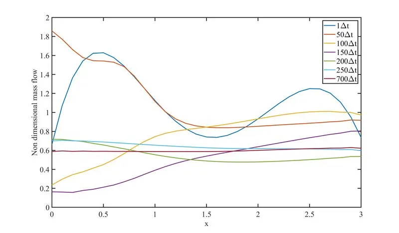
Figure: Variation of non-dimensional mass flow as funciton of distance through the nozzle (non conservative case)

From the above figure it is seen that the mass flow disturbance is very high for 1 and 50`\delta t` which settles down to a uniform value by 700`\delta t`.

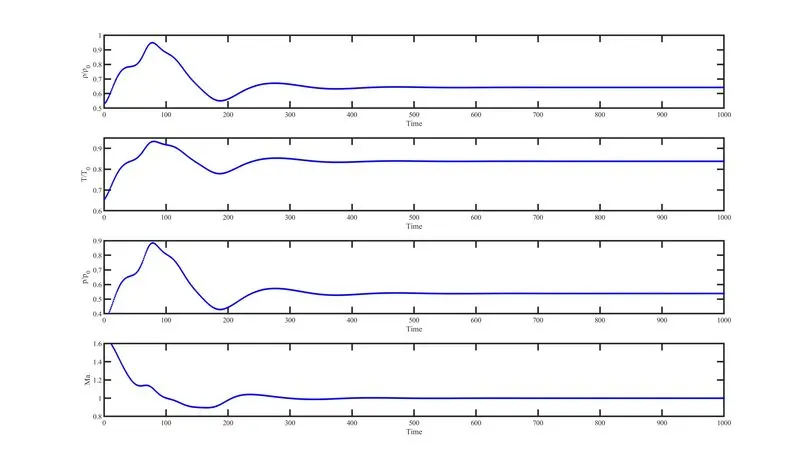
Figure: Time wise variation of density, temperstrue, pressure and Mach number (at `x=1.5`)

From the above figure it can be seen that the highest variations takes place the start of the iterations and after which the variables reach steady state variation asymptotically. This shows the rubber band effect.

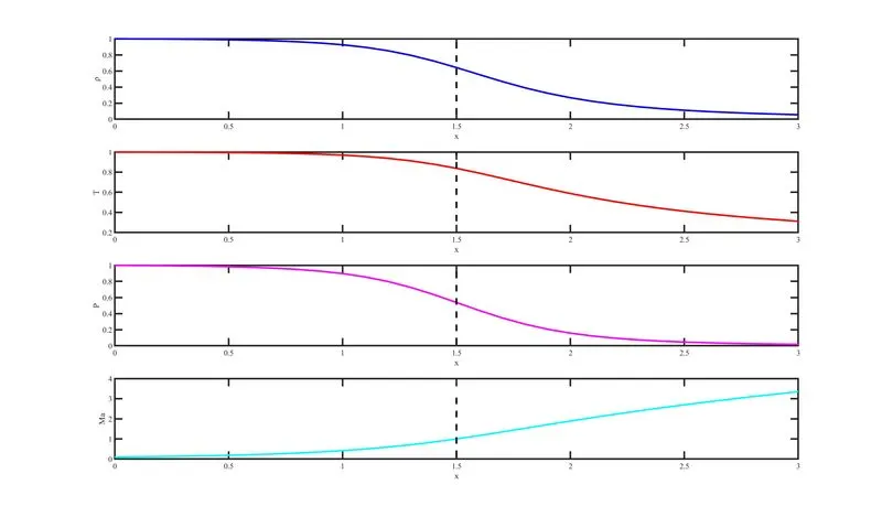
Figure: Variation of primitive variables as function of nozzle length at steady state.

Results of conservative form:

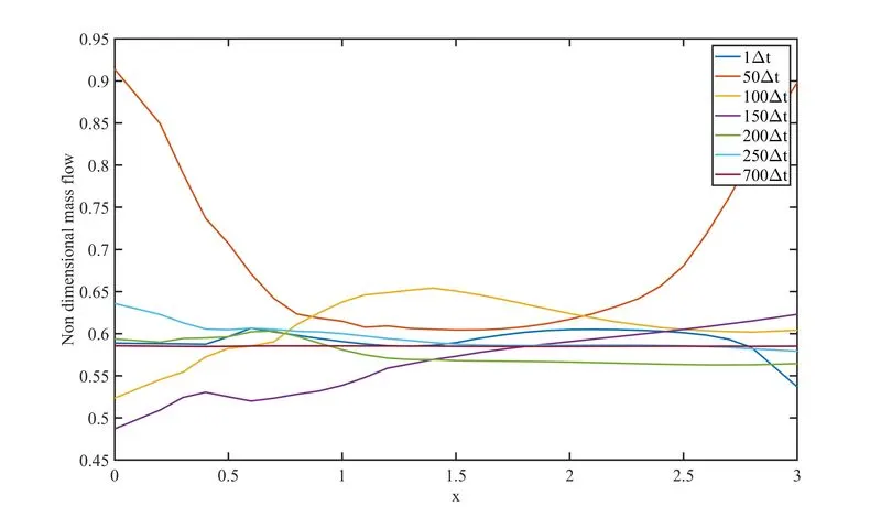
Figure: Variation of non-dimensional mass flow as funciton of distance through the nozzle (conservative case)

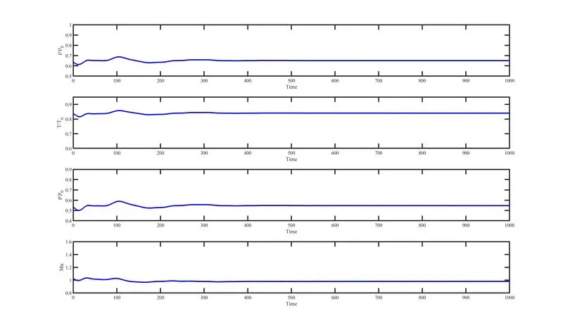
Figure: Time wise variation of density, temperstrue, pressure and Mach number (at `x=1.5`) (conservative case)

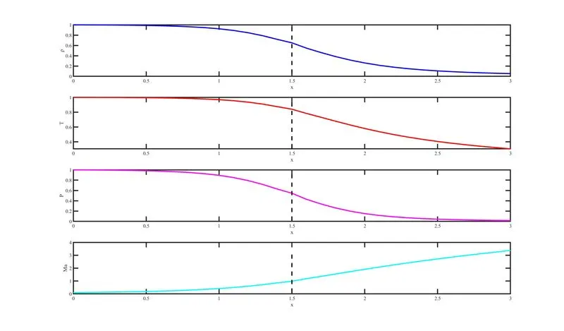
Figure: Variation of primitive variables as function of nozzle length at steady state (conservative case)

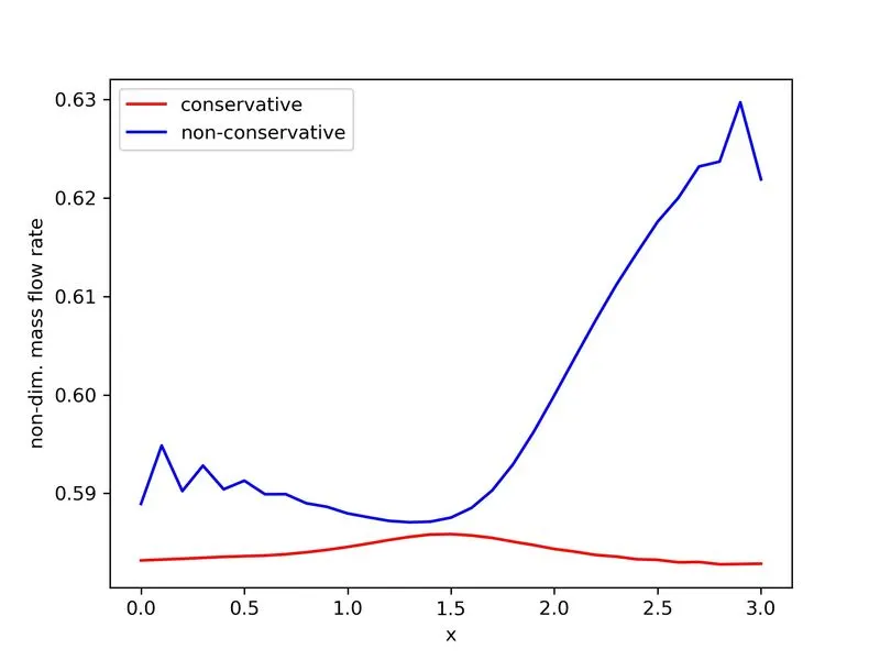
Figure: comparison of steady state mass flow for both conservative and non-conservative case

This show that the variation in the mass flow rate is much less sevier in case of conservative than non-conservative. From here two conclusions can be drawn:

1. Conservative form gives distribution much closer to a constant whereas, the nonconservation results have a considerable variation (One can see the oscillations at inler and outle).
2. The conservative form gives results more colse to the exact mass flow of 0.59.

Grid independence test for non-conservative case

pthon code

from pandas import *
inp=['T/T_0','ρ/ρ_0','p/p_0','Ma']
d_31=[0.8380301834357727, 0.6421334307583098, 0.5381271967686284, 0.9995004615632413]
d_61=[0.8371515789779461, 0.6412250158225623, 0.5368025344760166, 0.9992166920214245]

d = {
    'Output variable':inp,
    '31 points':d_31,
    '61 points':d_61
}
df=DataFrame(d)
df

Results:

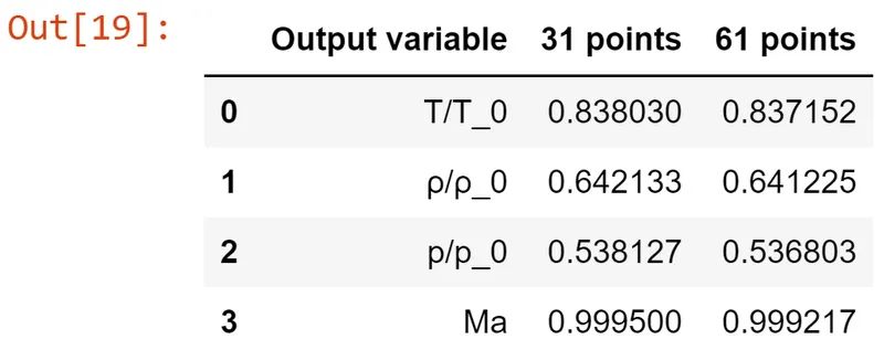
It has been observed that by doubling the number of grid the results are only marginally imporved hence the two results are almost the same. Hence, we can say that the original result at grid size of 31 is grid independent.