Week 5.1 - Mid term project - Solving the steady and unsteady 2D heat conduction problem
Figure 1. shows the 2D domain in which the problem must be solved. The boundary conditions are presented in the Figure itself. The problem is to solve steady and unsteady heat conduction equation in the domain. First, we will attempt the steady problem. (Note: horizontal axis is x and vertical axis is y)
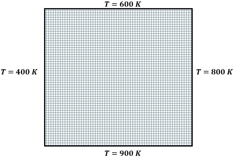
Figure1: Domain definition and boundary conditions
'Steady heat conduction analysis'
The 2D steady state heat conduction equation is written as:
`(\partial^2 T)/(\partial x^2)+(\partial^2 T)/(\partial y^2)=0`
Discretizing it using second order central differencing scheme will lead to:
`\frac{T_{i,j+1}-2T_{i,j}+T_{i,j-1}}{\Delta x^2}+\frac{T_{i-1,j}-2T_{i,j}+T_{i+1,j}}{\Delta x^2}=0`
(Note: I have use index `i` for rows and `j` for columns)
Bringing `T_{i,j}` terms on the left hand side we get:
`T_{i,j}=(1/a_P)\times(Hm+Vm)` (1)
where, `a_P=2/(Δx^2)+2/(Δy^2)`, `Hm=(T_{i,j+1}+T_{i,j-1})/(Δx^2)`, and `Vm=(T_{i-1,j}+T_{i+1,j})/(Δy^2)`
Equation 1 has to be solved on all the interior nodes by iterative method. In iterative methods we first guess the dependent variable throughout the domain. Then we iterate the domain point by point using above guesses. Then comparing the guessed value and value obtained after iteration and obtaining the error. If the error is more than a certain convergence criterion then we iterate again otherwise we say that the desired output is obtained. There are 3 famous iterative methods
- Jacobi
- Gauss-Seidel
- Successive over relaxation (SOR)
In Jacobi method the iteration uses the guessed value or the value from the previous iteration and the swipe through the domain then the new value become the guess for the next iteration till the convergence is achieved. Whereas, in case of Gauss-Seidel the iteration uses the current value of variable and swipe the domain that is the reason why it is faster than the Jacobi. In case of SOR we use a relaxation factor (`\beta`) to speed up the calculation further by updating more than what Gauss-Seidel does by a factor of `\beta`.
equation 1 when subject to all the iterative methods takes the form as follows:
| Iterative method | Mathematical representation | Matlab representation |
|
Jacobi |
`T_{i,j}=(1/a_P)\times(Hm+Vm)` `a_P=2/(Δx^2)+2/(Δy^2)` `Hm=(T_{i,j+1}+T_{i,j-1})/(Δx^2)` `Vm=(T_{i-1,j}+T_{i+1,j})/(Δy^2)` |
Hm=(T_old(i,j+1)+T_old(i,j-1))/dx^2; Vm=(T_old(i-1,j)+T_old(i+1,j))/dy^2; T(i,j)=(1.0/a_P)*(Hm+Vm); |
|
Gauss-Seidel |
`\beta=1` `Hm=(T(i,j+1)+T(i,j-1))/(\Deltax^2)` `Vm=(T(i-1,j)+T(i+1,j))/(\Deltay^2)` |
rf=1 Hm=(T(i,j+1)+T(i,j-1))/dx^2; |
|
Successive over relaxation (SOR) |
`\beta=1.7` `Hm=(T(i,j+1)+T(i,j-1))/(\Deltax^2)` `Vm=(T(i-1,j)+T(i+1,j))/(\Deltay^2)` |
rf=1.7 Hm=(T(i,j+1)+T(i,j-1))/dx^2; |
While writing the code no separate equation has been written for Gauss-seidel as the SOR gets converted to Gauss-Seidel when `\beta` becomes 1. Although `\beta` varies between 0 to 2 it should be less than 2. Normally over relaxation has been used for linear PDE's whereas for non-linear PDE's under relaxation is used. After hit and try we have arrived at `\beta=1.7` which gives result's very quickly i.e. with lesser number of iterations. During the code convergence criterion is set at `10^{-4}`.
Python code Implicit Steady State
from pylab import *

ℓx=1.0
ℓy=1.0

nc=20
nr=20

Δx=ℓx/(nc-1)
Δy=ℓy/(nr-1)

a_P=(2/Δx**2+2/Δy**2)

x=linspace(0,ℓx,nc)
y=linspace(0,ℓy,nr)

[X,Y]=meshgrid(x,flipud(y))

T=zeros((nr,nc))
T[0,:]=600.0
T[-1,:]=900.0
T[:,0]=400.0
T[:,-1]=800.0

T_old=T.copy()

print('which iterative solver you want to impliment')
scheme=input("for gauss seidel press 'g', for SOR 's' and for Jacobi 'j'\n")

error=1
ϵ=1.E-4
count=1
while error>ϵ:
    for i in range(1,nr-1):
        for j in range(1,nc-1):
            if scheme=='j' : ## Jacobi
                Hm=(T_old[i,j+1]+T_old[i,j-1])/Δx**2
                Vm=(T_old[i-1,j]+T_old[i+1,j])/Δy**2
                T[i,j]=(1/a_P)*(Hm+Vm)
            else:  ## Gauss and SOR
                if scheme=='g': # Gauss
                    β=1.0
                else:           # SOR
                    β=1.7

                Hm=(T[i,j+1]+T[i,j-1])/Δx**2
                Vm=(T[i-1,j]+T[i+1,j])/Δy**2
                T[i,j]=T_old[i,j]+(β/a_P)*(Hm+Vm-a_P*T_old[i,j])


    error=sum(abs(T-T_old))
    figure(1)
    if count%100==0:
        semilogy(count,error,'ko')
        print(count,'\t',error)

    T[0,:]=600.0
    T[-1,:]=900.0
    T[:,0]=400.0
    T[:,-1]=800.0

    T_old=T.copy()
    count=count+1


figure(2,dpi=300)
contourf(X,Y,T,12,cmap='jet')
xlabel('x')
ylabel('y')
colorbar()


show()
Matlab Code Implicit Steady State
% This code is to generate temperture field
% in steady state heat conduction.
% The method used in Implicit one

clear all
close all
clc

% Domain definition and grid generation

lx=1.0;
ly=1.0;

nc=20;
nr=20;

dx=lx/(nc-1);
dy=ly/(nr-1);

a_P=(2/dx^2+2/dy^2);

x=linspace(0,lx,nc);
y=linspace(0,ly,nr);

[X,Y]=meshgrid(x,fliplr(y));

% Initial guess and boundary conditions
T=zeros(nr,nc);
T(1,:)=600.0;
T(end,:)=900.0;
T(:,1)=400.0;
T(:,end)=800.0;

T_old=T;

% Scheme selector
disp('which iterative solver you want to impliment')
scheme=input("for gauss seidel press 2,..." + ...
    " for SOR 3 and for Jacobi 1\n")

error=1;
eps=1.e-4;
count=1;

while (error> eps)
    for i = 2:(nr-1)
        for j = 2:(nc-1)
            if (scheme==1)  % Jacobi
                Hm=(T_old(i,j+1)+T_old(i,j-1))/dx^2;
                Vm=(T_old(i-1,j)+T_old(i+1,j))/dy^2;
                T(i,j)=(1.0/a_P)*(Hm+Vm);

            else  % Gauss and SOR
                if (scheme==2) % Gauss
                    rf=1.0;    % rf : Relaxation Factor
                else           %SOR
                    rf=1.7;
                end


                Hm=(T(i,j+1)+T(i,j-1))/dx^2;
                Vm=(T(i-1,j)+T(i+1,j))/dy^2;
                T(i,j)=T_old(i,j)+(rf/a_P)*(Hm+Vm-a_P*T_old(i,j));
            end
        end
    end

    error=sum(sum(abs(T-T_old)));
    figure(1)
    if (mod(count,10)==0)
        semilogy(count,error,'ko');
        xlabel('iteration')
        ylabel('Error')
        hold on
        fprintf("%d,'\t',%f",count,error);
    end
     T(1,:)=600.0;
     T(end,:)=900.0;
     T(:,1)=400.0;
     T(:,end)=800.0;

    T_old=T;
    count=count+1;
end


 %Corner correction
 T(1,1)=(T(1,2)+T(2,2))/2
 T(end,1)=(T(end,2)+T(end-1,2))/2
 T(1,end)=(T(1,end-1)+T(2,end))/2
 T(end,end)=(T(end-1,end)+T(end,end-1))/2

if scheme==1
    name='Jacobi'
elseif scheme==2
    name='gauss-seidel'
else
    name='SOR'
end

figure(2)
[C,h]=contourf(X,Y,T,10)
hold on
clabel(C,h,'FontSize',15,'Color','k')
colormap('jet')
colorbar()
xlabel('x')
ylabel('y')
title_text=sprintf('Iteration count= %d, Iteration method=%s' ,count,name)
title(title_text)
Results and Discussion for steady implicit problem
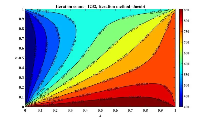
Figure 2: Contour plot for Jacobi iteration
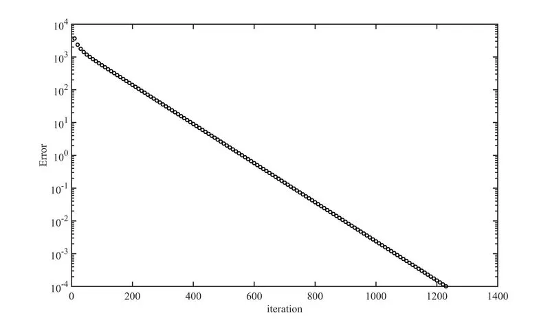
Figure 3: Error plot when Jacobi is used
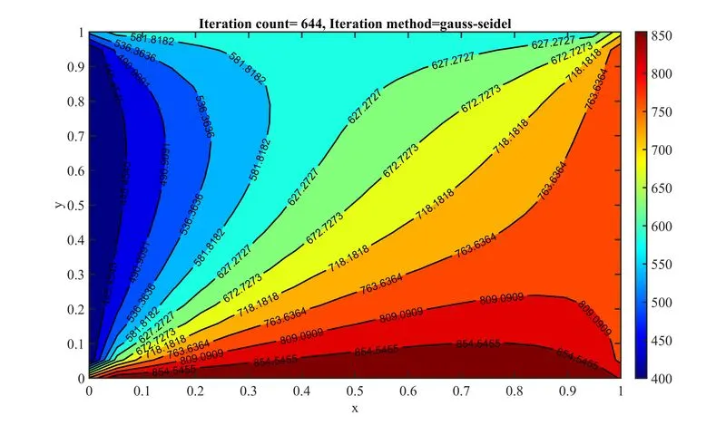
Figure 4: Contour plot for Gauss-Seidel iteration
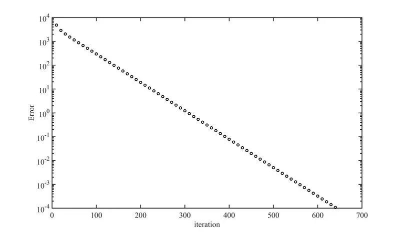
Figure 5: Error plot when Gauss-Seidel is used
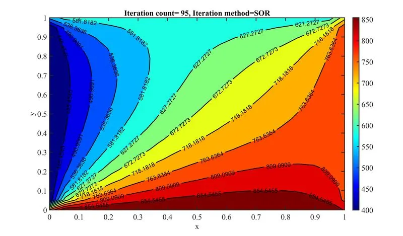
Figure 6: Contour plot for SOR iteration
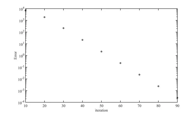
Figure 7: Error plot when SOR is used
For a grid size of 20`\times`20 the number of iterations for Jacobi, Gauss-Seidel, and SOR are 1232, 644, and 95, respectively. This proves that the SOR iteration technique 92.29 and 85% lesser iterations than Jacobi and SOR iterations. This is because of higher updation rate in SOR in comparison to others.
'Unsteady heat conduction analysis'
The 2D unsteady state heat conduction equation is written as:
`(1/\alpha)(\partialT)/(\partial t)=(\partial^2 T)/(\partial x^2)+(\partial^2 T)/(\partial y^2)`
Discretizing it using second order central differencing scheme for sapce and forward in time will lead to:
`(1/\alpha)\frac{T_i^{n+1}-T_i^n}{\Delta t}=\frac{T_{i,j+1}-2T_{i,j}+T_{i,j-1}}{\Delta x^2}+\frac{T_{i-1,j}-2T_{i,j}+T_{i+1,j}}{\Delta x^2}`
(Note: I have use index `i` for rows and `j` for columns )
Now the RHS can be evaluated at either `n`or `{n+1}^{th}` time step.
If it is evaluated at `n` time step the scheme is called as explicit otherwise (i.e., at `n+1^{th}` step) it is called as explicit scheme.
Bringing `T_{i,j}^{n+1}` terms on the left hand sides the implicit and explicit schemes becomes:
| Implicit | Explicit |
|
`k_1=alpha*(\Deltat)/(\Deltax^2)` Jacobi `Hm=T_{old_(i,j+1)}+T_{old_(i,j-1)}` Gauss-Seidel and SOR `\beta=1`- Gauss-Seidel `\beta=1.7`- SOR `Hm=T_{(i,j+1)}+T_{(i,j-1)}` |
`Hd=T_(i,j+1)-2T_(i,j)+T_(i,j-1)` |
In case of explicit algorithm with the initial conditions the problem march the domain point by point and evaluate the answer at each time step. The evaluation of time step is very crucial in explicit time marching problem. This is obtained with the help of CFL condition, which is mentioned as below:
`dd=1/(\Deltax^2)+1/(\Deltay^2); \Deltat<(0.5/alpha)\times(1/(dd));`
so, we have used 0.45 (in Explicit case) as the multiplying factor which has resulted in the time step as:
`\Deltat=(0.45/alpha)\times(1/(dd))`
`\alpha ` is considered as 0.1 and total time is considered as 40 sec.
As in implicit case time step does not pose any problem so 1 sec is chosen as time step.
Matlab Code Explict Unsteady state
% This code is to generate temperture field
% in Unsteady heat conduction using explicit scheme.
clear all
close all
clc

Lx=1.0;
Ly=1.0;
T=40.0; % Seconds

nc=20;
nr=20;

dx=Lx/(nc-1);
dy=Ly/(nr-1);

alpha=0.1;

%CFL condition

dd=1/dx^2+1/dy^2;
dt=(0.45/alpha)*(1/dd);
nt=int64(T/dt+1);

a_P=(2/dx^2+2/dy^2);

x=linspace(0,Lx,nc);
y=linspace(0,Ly,nr);

[X,Y]=meshgrid(x,fliplr(y));

T=zeros(nr,nc)+200; % Initial temperature field
T(1,:)=600.0;
T(end,:)=900.0;
T(:,end)=400.0;
T(:,end)=800.0;

T_old=T;

count=0;
tic
while count<=nt
    for i = 2:(nr-1)
        for j = 2:(nc-1)
            Hd=T(i,j+1)-2*T(i,j)+T(i,j-1);
            Vd=T(i-1,j)-2*T(i,j)+T(i+1,j);
            T(i,j)=T_old(i,j)+(alpha*dt/dx^2)*(Hd+Vd);
        end
    end
    T_old=T;
    count=count+1;
end
duration=toc
 %Corner correction
 T(1,1)=(T(1,2)+T(2,2))/2;
 T(end,1)=(T(end,2)+T(end-1,2))/2;
 T(1,end)=(T(1,end-1)+T(2,end))/2;
 T(end,end)=(T(end-1,end)+T(end,end-1))/2;

figure(1)
[C,h]=contourf(X,Y,T,10) ;
hold on
clabel(C,h,'FontSize',15,'Color','k');
colormap('jet');
xlabel('x');
ylabel('y');
colorbar();
title_text=sprintf('Time elapsed=%f, Time steps=%d' ,duration,count);
title(title_text);
Python Code Explict Unsteady state
from pylab import *

ℓx=1.0
ℓy=1.0
T=40.0 # Seconds

nc=20
nr=20

Δx=ℓx/(nc-1)
Δy=ℓy/(nr-1)

α=0.1

#CFL condition

dd=1/Δx**2+1/Δy**2
Δt=(0.45/α)*(1/dd)
nt=int(T/Δt+1)

a_P=(2/Δx**2+2/Δy**2)

x=linspace(0,ℓx,nc)
y=linspace(0,ℓy,nr)

[X,Y]=meshgrid(x,flipud(y))

T=zeros((nr,nc))+200
T[0,:]=600.0
T[-1,:]=900.0
T[:,0]=400.0
T[:,-1]=800.0

T_old=T.copy()

count=0
while count<=nt:
    for i in range(1,nr-1):
        for j in range(1,nc-1):
            Hd=T[i,j+1]-2*T[i,j]+T[i,j-1]
            Vd=T[i-1,j]-2*T[i,j]+T[i+1,j]
            T[i,j]=T_old[i,j]+(α*Δt/Δx**2)*(Hd+Vd)

    T_old=T.copy()
    count=count+1

figure(2,dpi=300)
contourf(X,Y,T,12,cmap='jet')
xlabel('x')
ylabel('y')
colorbar()
print(count)

show()
Results of Explict unsteady case
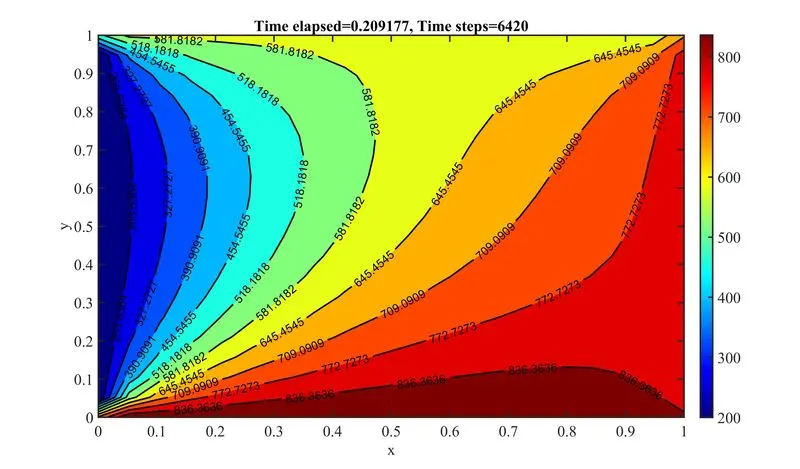
Figure 8: Contour plot for SOR iteration
Matlab Code Implicit Unsteady state
% This code is to generate temperture field
% in steady state heat conduction.
% The method used in Implicit one
clear all
close all
clc


Lx=1.0;
Ly=1.0;
T=40.0; % Seconds

nc=20;
nr=20;

dx=Lx/(nc-1);
dy=Ly/(nr-1);

alpha=0.1;


dt=1;
nt=int64(T/dt+1);
fprintf('Total time steps=%d',nt);
k1=alpha*dt/dx^2;
k2=alpha*dt/dy^2;


x=linspace(0,Lx,nc);
y=linspace(0,Ly,nr);

[X,Y]=meshgrid(x,fliplr(y));

T=zeros(nr,nc)+200; % Initial conditions
T(1,:)=600.0;
T(end,:)=900.0;
T(:,1)=400.0;
T(:,end)=800.0;

T_prev=T;
T_old=T;

disp('which iterative solver you want to impliment');
scheme=input("for gauss seidel press 2, for SOR 3 and for Jacobi 1\n");


% Time loop
tic
for tau = 1:nt

% Iteration loop
    error=1;
    count_inner=1;

    while error>0.0001
        for i = 2:nr-1
            for j = 2:nc-1
                if scheme==1  % Jacobi
                    Hm=T_old(i,j+1)+T_old(i,j-1);
                    Vm=T_old(i-1,j)+T_old(i+1,j);
                    T(i,j)=(T_prev(i,j)+k1*Hm+k2*Vm)/(1+2*k1+2*k2);
                else  % Gauss and SOR
                    if scheme==2 % Gauss
                        beta=1.0;
                    else           % SOR
                        beta=1.7;
                    end

                    Hm=T(i,j+1)+T(i,j-1);
                    Vm=T(i-1,j)+T(i+1,j);
                    T(i,j)=(T_prev(i,j)+k1*Hm+k2*Vm)/(1+2*k1+2*k2);
                    T(i,j)=T_old(i,j)+beta*(T(i,j)-T_old(i,j));
                end
            end
        end
        error=sum(sum(abs(T-T_old)));

        T(1,:)=600.0;
        T(end,:)=900.0;
        T(:,1)=400.0;
        T(:,end)=800.0;

        T_old=T;
        count_inner=count_inner+1;
    T_prev=T;
    fprintf('tau=%d and count_iter=%d\n',tau,count_inner);
    end
end

if scheme==1
    name='Jacobi'
elseif scheme==2
    name='gauss-seidel'
else
    name='SOR'
end


%Corner correction
 T(1,1)=(T(1,2)+T(2,2))/2;
 T(end,1)=(T(end,2)+T(end-1,2))/2;
 T(1,end)=(T(1,end-1)+T(2,end))/2;
 T(end,end)=(T(end-1,end)+T(end,end-1))/2;


duration=toc;
figure(1)
[C,h]=contourf(X,Y,T,10) ;
hold on
clabel(C,h,'FontSize',15,'Color','k');
colormap('jet');
xlabel('x');
ylabel('y');
colorbar();
title_text=sprintf('Time elapsed=%f, Iteration method=%s' ,duration,name);
title(title_text);
Python Code Implicit Unsteady state
from pylab import *
from time import *
ℓx=1.0
ℓy=1.0
T=40.0 # Seconds

nc=20
nr=20

Δx=ℓx/(nc-1)
Δy=ℓy/(nr-1)

α=0.1

#dd=1/Δx**2+1/Δy**2
#Δt=0.4*α*(1/dd)
Δt=4
nt=int(T/Δt+1)
print('Total time steps=',nt)
k1=α*Δt/Δx**2
k2=α*Δt/Δy**2


x=linspace(0,ℓx,nc)
y=linspace(0,ℓy,nr)

[X,Y]=meshgrid(x,flipud(y))

T=zeros((nr,nc))+200
T[0,:]=600.0
T[-1,:]=900.0
T[:,0]=400.0
T[:,-1]=800.0

T_prev=T_old=T.copy()

print('which iterative solver you want to impliment')
scheme=input("for gauss seidel press 'g', for SOR 's' and for Jacobi 'j'\n")


# Time loop
start=time()
for τ in range(nt):

# Iteration loop
    error=1
    count_inner=1

    while error>0.0001:
        for i in range(1,nr-1):
            for j in range(1,nc-1):
                if scheme=='j' : ## Jacobi
                    Hm=(T_old[i,j+1]+T_old[i,j-1])
                    Vm=(T_old[i-1,j]+T_old[i+1,j])
                    T[i,j]=(T_prev[i,j]+k1*Hm+k2*Vm)/(1+2*k1+2*k2)
                else:  ## Gauss and SOR
                    if scheme=='g': # Gauss
                        β=1.0
                    else:           # SOR
                        β=1.7

                    Hm=(T[i,j+1]+T[i,j-1])
                    Vm=(T[i-1,j]+T[i+1,j])
                    T[i,j]=(T_prev[i,j]+k1*Hm+k2*Vm)/(1+2*k1+2*k2)
                    T[i,j]=T_old[i,j]+β*(T[i,j]-T_old[i,j])
        error=sum(abs(T-T_old))

        T[0,:]=600.0
        T[-1,:]=900.0
        T[:,0]=400.0
        T[:,-1]=800.0

        T_old=T.copy()
        count_inner=count_inner+1
    T_prev=T.copy()
    print('τ',τ,'\t',count_inner)
contourf(X,Y,T,12,cmap='jet')
xlabel('x')
ylabel('y')
show()
stop=time()
duration=stop-start
print('Duration=',duration)
Results of Implicit unsteady case
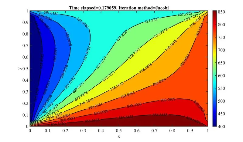
Figure 9 Contour plot for Jacobi iteration (Implicit unsteady)
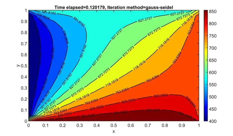
Figure 10 Contour plot for Gauss-Seidel iteration (Implicit unsteady)
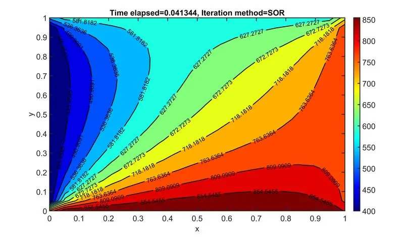
Figure 11 Contour plot for SOR iteration (Implicit unsteady)
With SOR the time taken by the code is only 0.041344 sec whereas, for Jacobi and Gauss-Seidel it takes 0.179054 and 0.120179 sec. respectively.
All the contours look the same because the problem is the same. The underlying physics behind the solution is that the diffusion of temperature is happening from higher temperature regions to the lower and finally for a fixed boundary conditions the domain acquire a steady state.