Week 3.5 - Deriving 4th order approximation of a 2nd order derivative using Taylor Table method

Derivation of the 4^th order approximations of the second-order derivative, the code to evaluate the coefficients, and the output are as follows:

Central Difference

`N=P+Q-1=4+2-1=5`

Total 5 terms will be there out of which one is and remaining 4 will be equally distributed on both side of it (i.e., 2 on left and 2 on right).

`f^'' (i)Δx^2=af_(i-2)+bf_(i-1)+cf_(i)+df_(i+1)+ef_(i+2)`

	`f(i)`	`f^' (i)Δx `	`f^'' (i)Δx^2`	`f^(''') (i)Δx^3`	`f^'''' (i)Δx^4`
`a f_(i-2)`	a	-2a	(4/2)a	-(8/6)a	(16/24)a
`b f_(i-1)`	b	-b	(1/2)b	-(1/6)b	(1/24)b
`c f_i`	c	0	0	0	0
`d f_(i+1)`	d	d	(1/2)d	(1/6)d	(1/24)d
`e f_(i+2)`	e	2e	(4/2)e	(8/6)e	(16/24)e
	0	0	1	0	0

Skewed righ-sided difference

`N=P+Q=4+2=6`

Total 6 terms will be there out of which one is and remaining 5 will on right of it.

`f^'' (i)Δx^2=af_i+bf_(i+1)+cf_(i+2)+df_(i+3)+ef_(i+4)+gf_(i+5)`

	`f(i)`	`f^' (i)Δx `	`f^'' (i)Δx^2`	`f^(''') (i)Δx^3`	`f^'''' (i)Δx^4`	`f^''''' (i)Δx^5`
`a f_i`	a	0	0	0	0	0
`b f_(i+1)`	b	b	(1/2)b	(1/6)b	(1/24)b	(1/120)b
`c f_(i+2)`	c	2c	(4/2)c	(8/6)c	(16/24)c	(32/120)c
`d f_(i+3)`	d	3d	(9/2)d	(27/6)d	(81/24)d	(243/120)d
`e f_(i+4)`	e	4e	(16/2)e	(64/6)e	(256/24)e	(1024/120)e
`g f_(i+5)`	g	5g	(25/2)g	(125/6)g	(625/24)g	(3125/120)g
	0	0	1	0	0	0

Skewed left-sided difference

`N=P+Q=4+2=6`

Total 6 terms will be there out of which one is and remaining 5 will on left of it.

`f^'' (i)Δx^2=af_(i-5)+bf_(i-4)+cf_(i-3)+df_(i-2)+ef_(i-1)+gf_i`

	`f(i)`	`f^' (i)Δx `	`f^'' (i)Δx^2`	`f^(''') (i)Δx^3`	`f^'''' (i)Δx^4`	`f^''''' (i)Δx^5`
`a f_(i-5)`	a	5a	(25/2)a	(125/6)a	(625/24)a	(3125/120)a
`b f_(i-4)`	b	4b	(16/2)b	(64/6)b	(256/24)b	(1024/120)b
`c f_(i-3)`	c	3c	(9/2)c	(27/6)c	(81/24)c	(243/120)c
`d f_(i-2)`	d	2d	(4/2)d	(8/6)d	(16/24)d	(32/120)d
`e f_(i-1)`	e	e	(1/2)e	(1/6)e	(1/24)e	(1/120)e
`g f_i`	g	0	0	0	0	0
	0	0	1	0	0	0

Matlab Program to evaluate coefficients

clear all
close all
clc

%% Central Difference
Ac=[
    1,1,1,1,1;
    -2,-1,0,1,2;
    2,1/2,0,1/2,2;
    -4/3,-1/6,0,1/6,4/3;
    2/3,1/24,0,1/24,2/3
    ];
Bc=[0;0;1;0;0];
xc=linsolve(Ac,Bc);



%% Skewed Right
Ar=[
        1,1,1,1,1,1;
        0,1,2,3,4,5;
        0,1/2,4/2,9/2,16/2,25/2;
        0,1/6,8/6,27/6,64/6,125/6;
        0,1/24,16/24,81/24,256/24,625/24;
        0,1/120,32/120,243/120,1024/120,3125/120
        ];
Br=[0;0;1;0;0;0];
xr=linsolve(Ar,Br);


%% Skewed Left

Al=[     1,1,1,1,1,1;
        5,4,3,2,1,0;
        25/2,16/2,9/2,4/2,1/2,0;
        125/6,64/6,27/6,8/6,1/6,0;
        625/24,256/24,81/24,16/24,1/24,0;
        3125/120,1024/120,243/120,32/120,1/120,0
  ];
Bl=[0;0;1;0;0;0];
xl=linsolve(Al,Bl);

% Printing coefficients

% Central
coefficients = {'a';'b';'c';'d';'e'};
values = xc;
Central_difference = table(coefficients,values)

% Right
coefficients = {'a';'b';'c';'d';'e';'g'};
values = xr;
Right_skewed = table(coefficients,values)

% Left
coefficients = {'a';'b';'c';'d';'e';'g'};
values = xl;
Left_skewed = table(coefficients,values)

Program Output

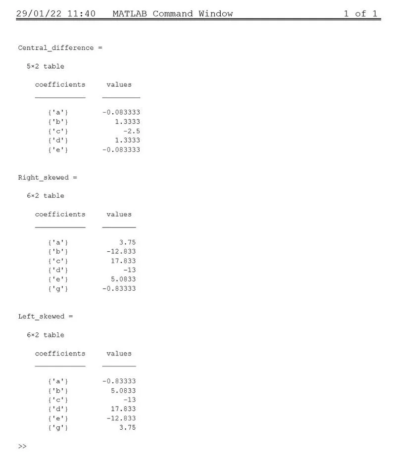
Now it’s time to check the progress of central, left and right skewed differences in contrast to the exact derivative of following function:

`e^x cos(x)`

Following Matlab program has been developed to evaluate the exact and all the differences for varying value of the grid size which is ranging from 1/1000 to 1 with 50 equal intervals in between and considering x=`\pi`:

clear all
close all
clc

%% Central Difference
Ac=[
    1,1,1,1,1;
    -2,-1,0,1,2;
    2,1/2,0,1/2,2;
    -4/3,-1/6,0,1/6,4/3;
    2/3,1/24,0,1/24,2/3
    ];
Bc=[0;0;1;0;0];
xc=linsolve(Ac,Bc);



%% Skewed Right
Ar=[
        1,1,1,1,1,1;
        0,1,2,3,4,5;
        0,1/2,4/2,9/2,16/2,25/2;
        0,1/6,8/6,27/6,64/6,125/6;
        0,1/24,16/24,81/24,256/24,625/24;
        0,1/120,32/120,243/120,1024/120,3125/120
        ];
Br=[0;0;1;0;0;0];
xr=linsolve(Ar,Br);


%% Skewed Left

Al=[     1,1,1,1,1,1;
        5,4,3,2,1,0;
        25/2,16/2,9/2,4/2,1/2,0;
        125/6,64/6,27/6,8/6,1/6,0;
        625/24,256/24,81/24,16/24,1/24,0;
        3125/120,1024/120,243/120,32/120,1/120,0
  ];
Bl=[0;0;1;0;0;0];
xl=linsolve(Al,Bl);


%% Exact
x=pi;
dx=linspace(1/1000,1,50);

exact=-2*sin(x)*exp(x)

d2f_dx2_cd=zeros(length(dx),1);
d2f_dx2_rs=zeros(length(dx),1);
d2f_dx2_ls=zeros(length(dx),1);

for i=1:length(dx)
% Central diff
d2f_dx2_cd(i)=(xc(1)*f(x-2*dx(i))+xc(2)*f(x-dx(i))+xc(3)*f(x)+xc(4)*f(x+dx(i))+...
    xc(5)*f(x+2*dx(i)))/dx(i)^2;
% Right Skewed
d2f_dx2_rs(i)=(xr(1)*f(x)+xr(2)*f(x+dx(i))+xr(3)*f(x+2*dx(i))+xr(4)*f(x+3*dx(i))+...
    xr(5)*f(x+4*dx(i))+xr(6)*f(x+5*dx(i)))/dx(i)^2;
% Left Skewed
d2f_dx2_ls(i)=(xl(1)*f(x-5*dx(i))+xl(2)*f(x-4*dx(i))+xl(3)*f(x-3*dx(i))+ ...
    xl(4)*f(x-2*dx(i))+xl(5)*f(x-dx(i))+xl(6)*f(x))/dx(i)^2;
end
%% Error evaluation
error_cd=abs(exact-d2f_dx2_cd)
error_rs=abs(exact-d2f_dx2_rs)
error_ls=abs(exact-d2f_dx2_ls)

%% Data Plotting
figure(1)
plot(dx,error_cd,'r-o')
hold on
plot(dx,error_ls,'g-o')
plot(dx,error_rs,'b-o')
xlabel('dx')
ylabel('error')
legend('central','left skewed','right skewed')

figure(2)
semilogy(dx,error_cd,'r-o')
hold on
semilogy(dx,error_ls,'g-o')
semilogy(dx,error_rs,'b-o')
xlabel('dx')
ylabel('error')
legend('central','left skewed','right skewed')



%% Function
function y=f(x);
        y=cos(x)*exp(x);
end

Results and Discussions

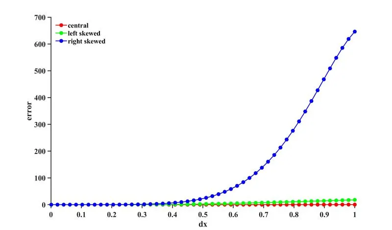
Figure 1: Error variation as a function of dx

It can be seen from Figure 1 that till step size of 0.3 the variation of error is very small but as the step size increases further the right skewed differencing shows a huge error with a very steep rise in the error line. The central and left skew differencing are more stable with less prone to the error with grid size. Moreover, the least amount of error is observed in case of central differencing.

To clear this picture more a semilogy graph has been drawn and shown in the Figure 2.

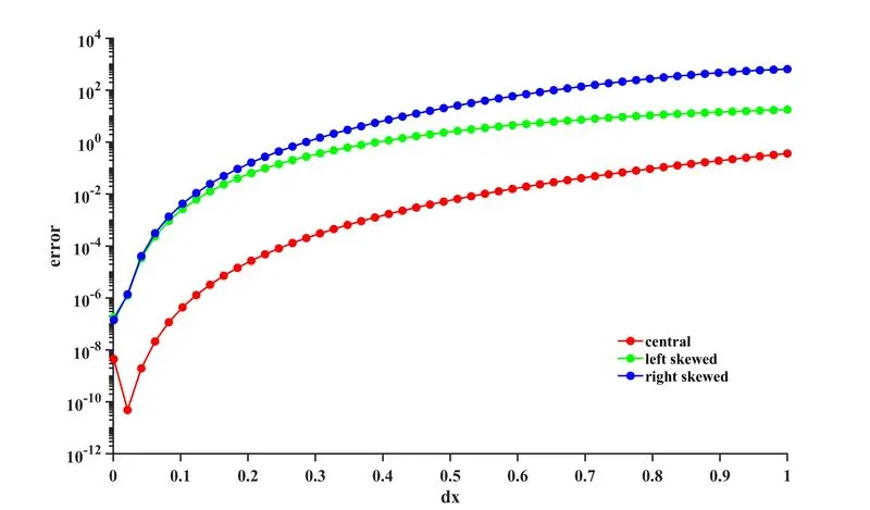
Figure 2: error variation on semilogy graph

From this figure is it is observed that though the error in central difference is least but there is a gradual rise in it is observed but the graph of left differencing has almost become flat.

Now to answer the last question it can be simply said that at the boundaries the central differencing cannot be used as there will not be any grid point outside the domain. In case of boundary nodes only skewed differencing methods can be used.