Week 7 - Simulation of a 1D Super-sonic nozzle flow simulation using Macormack Method

Objective:

To simulate the isentropic flow through a Quasi 1D subsonic nozzle by deriving both the conservation and non-conservation forms of the governing equations and solve them by implementing MacCormack's technique using MATLAB.

Problem:

1. We need to show the following plots inside your report
   Steady-state distribution of primitive variables inside the nozzle.
2. Time-wise variation of the primitive variables.
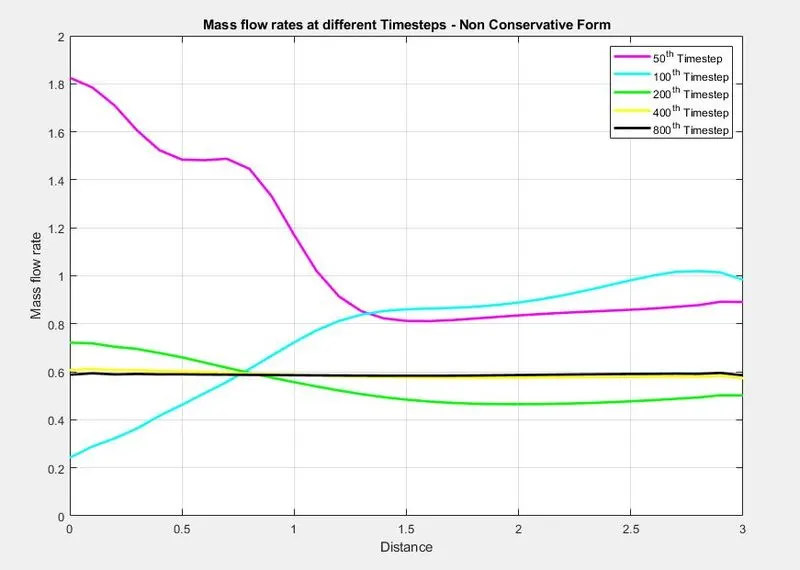
3. Variation of Mass flow rate distribution inside the nozzle at different time steps during the time-marching process.
4. Comparison of Normalized mass flow rate distributions of both forms.

Theory:

1-D Flow

A quasi-one-dimensional flow is one in which all variables vary primarily along one direction (say in the x-direction).

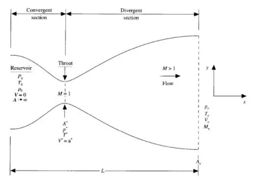
Nozzle Diagram

We consider the flow distribution only in the x-direction.

The flow at the inlet of the nozzle comes from the reservoir. The cross-section area of the reservoir is very large and hence velocity is very small. The flow is locally subsonic in the convergent section of the nozzle, and Sonic at the throat, and Supersonic at the divergent section.

Governing Equations

Non Conservative Form

(In this form, the control volume is moving)

Continuity Equation

`(delrho')/(delt') = -rho'((delV')/(delx')) -rho'V'((del(lnA'))/(delx')) - V'((delrho')/(delx'))`

Momentum Equation

`(delV')/(delt') = -V'((delV')/(delx')) - (1/(gamma))((delT')/(delx') + (T')/(rho')((delrho')/(delx')))`

Energy Equation

`(delT')/(delt') = -V'((delT')/(delx')) -(gamma-1)T'((delV')/(delx') + V'((del(lnA'))/(delx')))`

Conservative Form

(In this form, the control volume is stationary)

Continuity Equation

`(del(rho'A'))/(delt') + (del(rho'A'V'))/(delx') = 0`

Momentum Equation

`(del(rho'A'V'))/(delt') + (del(rho'A'(V')^2 + (1/gamma)rho'A'))/(delx') = (1/gamma)rho'((delA')/(delx'))`

Energy Equation

`(del(rho'((e')/(gamma-1) +((gamma)/2)(V')^2)A'))/(delt') + (del(rho'((e')/(gamma-1) +((gamma)/2)(V')^2)V'A' + rho'A'V'))/(delx') = 0`

For air at standard condition, `gamma = 1.4`

Non Dimensional Quantities

`T' = T/L, rho' = (rho')/(rho_0), x' = x/L`

`V' = V/a_0,` where `a_0`is speed of sound

`t' = t/(L/a_0), A' = A/(A')`

Macormack Method

To discretize the solution we use this method.

We will be doing time marching to solve.

This is done in two steps, A Predictor Step and then Corrector Step.

• Predictor Step

In this, we do forward differencing of space terms.

`((delf)/(delt))_P = (f(i+1) -f(i))/(Deltax)`

• Solution Update

`f_P = f_(Initial) + ((delf)/(delt))_P*(Deltat)`

• Corrector Step

`((delf)/(delt))_c = (f(i) -f(i-1))/(Deltax)`

`((delf)/(delt))_(avg) = 0.5(((delf)/(delt))_P + ((delf)/(delt))_c)`

• Final Solution Update

`f_(sol) = f_(Initial) + ((delf)/(delt))_(avg)*(Deltat)`

MATLAB CODE

Main Program Code

% Solving Quasi 1D supersonic nozzle flow equation
% For both Conservative and Non-Conservative form
% of governing equations

clear all
close all
clc

% Inputs
% number of grid points
% We take user input to change number of grids [31,62,93]
n = input('Number of grids: ');
l = 3;
x = linspace(0,l,n);
dx = x(2) - x(1);
gamma = 1.4;

% number of time step
nt = 1400;
% Courant Number
C = 0.5;

% Function for non-conservative form

tic;
[mass_flow_rate_NC, pressure_NC, mach_number_NC, rho_NC, v_NC, T_NC, rho_throat_NC, v_throat_NC, T_throat_NC, mass_flow_rate_throat_NC, pressure_throat_NC, mach_number_throat_NC] = non_conservative_form(x, dx, n, gamma, nt, C);
time_elapsed_NC = toc;

fprintf('Time Elasped for Non Conservative form: %0.4f\n', time_elapsed_NC);
hold on

% Plottings

% Timestep variation of properties at throat area for non-conservative form

figure(1)

% Density
subplot(4,1,1)
plot(linspace(1,nt,nt),rho_throat_NC)
ylabel('Density')
legend('Density at throat');
axis([0 1400 0 1.3]);
grid on;
title('Timestep variation at throat area - Non Conservative Form')

% Temperature
subplot(4,1,2)
plot(linspace(1,nt,nt),T_throat_NC)
ylabel('Temperature')
legend('Temperature at throat');
axis([0 1400 0.6 1]);
grid on;

% Pressure
subplot(4,1,3)
plot(linspace(1,nt,nt),pressure_throat_NC)
ylabel('Pressure')
legend('Pressure at throat');
axis([0 1400 0.4 1.1]);
grid on

% Mach Number
subplot(4,1,4)
plot(linspace(1,nt,nt),mach_number_throat_NC)
xlabel('Timesteps')
ylabel('Mach Number')
legend('Mach Number at throat');
axis([0 1400 0.6 1.4]);
grid on;

% Steady-state simulation for non-conservative form

figure(2);

% Density
subplot(4,1,1);
plot(x,rho_NC)
ylabel('Density')
legend({'Density'});
axis([0 3 0 1])
grid on;
title('Variation of Flow Rate Distribution-Non Conservative Form')

% Temperature
subplot(4,1,2);
plot(x,T_NC)
ylabel('Temperature')
legend({'Temperature'});
axis([0 3 0 1])
grid on;

% Pressure
subplot(4,1,3);
plot(x,pressure_NC)
ylabel('Pressure')
legend({'Pressure'});
axis([0 3 0 1])
grid on;

% Mach number
subplot(4,1,4);
plot(x,mach_number_NC)
xlabel('Nozzle Length')
ylabel('Mach number')
legend({'Mach number'});
axis([0 3 0 4])
grid on;

% Function for conservative form

tic;
[mass_flow_rate_C, pressure_C, mach_number_C, rho_C, v_C, T_C, rho_throat_C, v_throat_C, T_throat_C, mass_flow_rate_throat_C, pressure_throat_C, mach_number_throat_C] = conservative_form(x, dx, n, gamma, nt, C);

time_elasped_C = toc;

fprintf('Time Elasped for Conservative form: %d\n', time_elasped_C);

% Plotting

% Timestep variation of properties at throat area in Conservative form

figure(3)

% Density
subplot(4,1,1)
plot(linspace(1,nt,nt),rho_throat_C)
ylabel('Density')
legend({'Density at throat'});
axis([0 1400 0 1]);
grid on;
title('Timestep variation at throat area-Conservative form')

% Temperature
subplot(4,1,2)
plot(linspace(1,nt,nt),T_throat_C)
ylabel('Temperature')
legend({'Temperature at throat'});
axis([0 1400 0.6 1]);
grid on;

% Pressure
subplot(4,1,3)
plot(linspace(1,nt,nt),pressure_throat_C)
ylabel('Pressure')
legend({'Pressure at throat'});
axis([0 1400 0.2 0.8]);
grid on;

% Mach Number
subplot(4,1,4)
plot(linspace(1,nt,nt),mach_number_throat_C)
xlabel('Timesteps')
ylabel('Mach Number')
legend({'Mach Number at throat'});
axis([0 1400 0.6 1.4]);
grid on;

% Steady-state simulation for Non-Conservative form

figure(4);

% Density
subplot(4,1,1);
plot(x,rho_C)
ylabel('Density')
legend({'Density'});
axis([0 3 0 1])
grid on;
title('Variation of Flow Rate Distribution-Conservative form')

% Temperature
subplot(4,1,2);
plot(x,T_C)
ylabel('Temperature')
legend({'Temperature'});
axis([0 3 0 1])
grid on;

% Pressure
subplot(4,1,3);
plot(x,pressure_C)
ylabel('Pressure')
legend({'Pressure'});
axis([0 3 0 1])
grid on;

% Mach number
subplot(4,1,4);
plot(x,mach_number_C)
xlabel('Nozzle Length')
ylabel('Mach number')
legend({'Mach number'});
axis([0 3 0 4])
grid on;

% Comparison of Normalized mass flow rate distributions of both forms

figure(5)
plot(x,mass_flow_rate_NC,'r','linewidth',2)
hold on;
plot(x,mass_flow_rate_C,'b','linewidth',2)
hold on;
grid on
legend('Non Conservative Form','Conservative Form');
xlabel('Length of the Domain')
ylabel('Mass Flow Rate')
title('Comparison of Normalized mass flow rate of both forms')

% Grid independency test graphs
figure(8)
subplot(2,1,1)
plot(x, mass_flow_rate_NC)
hold on
xlabel('Time Steps')
ylabel('Mass flow rate')
title(['Non-Conservative Form: Grid independeancy test at throat at node, n = ',num2str(n)])

subplot(2,1,2)
plot(x, mass_flow_rate_C)
hold on
xlabel('Time Steps')
ylabel('Mass flow rate')
title(['Conservative Form: Grid independeancy test at throat at node, n = ',num2str(n)])

Explanation

• Input parameters are assigned for the variables x, dx, n, gamma, nt, and C.
• Non-Conservative and Conservative forms are created as separate functions with the necessary inputs.
• tic toc command is used for calculating the time elapsed between the functions.
• Then we plot for the following solutions

• Timestep variation at the throat area of both forms.
• Variation of Flow Rate Distribution of both forms.
• Comparison of Normalized Mass Flow Rate of both forms.

Function calling for Non- Conservative Form

% Function for Non-Conservative form

function [mass_flow_rate_NC, pressure_NC, mach_number_NC, rho_NC, v_NC, T_NC, rho_throat_NC, v_throat_NC, T_throat_NC, mass_flow_rate_throat_NC, pressure_throat_NC, mach_number_throat_NC] = non_conservative_form(x, dx, n, gamma, nt, C)

% Calculate intial profiles
rho_NC = 1 - 0.3146*x;
T_NC = 1 - 0.2341*x;
v_NC = (0.1 + 1.09*x).*T_NC.^0.5;

% Area
a = 1 + 2.2*(x - 1.5).^2;

% Outer time loop
for k = 1:nt
    %Time-step control
    dt = min(C.*dx./(sqrt(T_NC) + v_NC));
    
    % Saving a copy of Old Values
    rho_old = rho_NC;
    T_old = T_NC;
    v_old = v_NC;
    
    % Predictor method
    for j = 2:n-1
        % Simplifying the equation in simple terms
        dv_dx = (v_NC(j + 1) - v_NC(j))/dx;
        drho_dx = (rho_NC(j + 1) - rho_NC(j))/dx;
        dT_dx = (T_NC(j + 1) - T_NC(j))/dx;
        dlog_a_dx = (log(a(j + 1)) - log(a(j)))/dx;
        
        % Continuity equation
        drho_dt_P(j) = -rho_NC(j)*dv_dx - rho_NC(j)*v_NC(j)*dlog_a_dx - v_NC(j)*drho_dx;
        
        % Momentum equation
        dv_dt_P(j) = -v_NC(j)*dv_dx - (1/gamma)*(dT_dx + (T_NC(j)*drho_dx/rho_NC(j)));
        
        % Energy equation
        dT_dt_P(j) = -v_NC(j)*dT_dx - (gamma - 1)*T_NC(j)*(dv_dx + v_NC(j)*dlog_a_dx);
        
        %Solution Update
        rho_NC(j) = rho_NC(j) + drho_dt_P(j)*dt;
        v_NC(j) = v_NC(j) + dv_dt_P(j)*dt;
        T_NC(j) = T_NC(j) + dT_dt_P(j)*dt;
    end
    
    % Corrector method
    for j = 2:n-1
        %Simplifying the equation in simple terms
        dv_dx = (v_NC(j) - v_NC(j - 1))/dx;
        drho_dx = (rho_NC(j) - rho_NC(j - 1))/dx;
        dT_dx = (T_NC(j) - T_NC(j - 1))/dx;
        dlog_a_dx = (log(a(j)) - log(a(j - 1)))/dx;
        
        % Continuity equation
        drho_dt_C(j) = - rho_NC(j)*dv_dx - rho_NC(j)*v_NC(j)*dlog_a_dx - v_NC(j)*drho_dx;
        
        % Momentum equation
        dv_dt_C(j) = - v_NC(j)*dv_dx - (1/gamma)*(dT_dx + (T_NC(j)*drho_dx/rho_NC(j)));
        
        % Energy equation
        dT_dt_C(j) = - v_NC(j)*dT_dx - (gamma - 1)*T_NC(j)*(dv_dx + v_NC(j)*dlog_a_dx);
    end
    
    % Compute average time derivative
    drho_dt = 0.5.*(drho_dt_P + drho_dt_C);
    dv_dt = 0.5.*(dv_dt_P + dv_dt_C);
    dT_dt = 0.5.*(dT_dt_P + dT_dt_C);
    
    % Final solution update
    for i = 2:n-1
        rho_NC(i) = rho_old(i) + drho_dt(i)*dt;
        v_NC(i) = v_old(i) + dv_dt(i)*dt;
        T_NC(i) = T_old(i) + dT_dt(i)*dt;
    end  
    
    % Applying boundary conditions
    % Inlet
    rho_NC(1) = 1;
    v_NC(1) = 2*v_NC(2) - v_NC(3);
    T_NC(1) = 1;
    
    % Outlet
    rho_NC(n) = 2*rho_NC(n-1) - rho_NC(n - 2);
    v_NC(n) = 2*v_NC(n - 1) - v_NC(n - 2);
    T_NC(n) = 2*T_NC(n - 1) - T_NC(n - 2);
    
    % Defining Mass flow rate, Pressure and Mach number
    mass_flow_rate_NC = rho_NC.*a.*v_NC;
    pressure_NC = rho_NC.*T_NC;
    mach_number_NC = (v_NC./sqrt(T_NC));
    
    % Calculating Variables at throat section
    rho_throat_NC(k) = rho_NC(16);
    T_throat_NC(k) = T_NC(16);
    v_throat_NC(k) = v_NC(16);
    mass_flow_rate_throat_NC(k) = mass_flow_rate_NC(16);
    pressure_throat_NC(k) = pressure_NC(16);
    mach_number_throat_NC(k) = mach_number_NC(16);
    
    % Plotting
    % Comparison of non-dimensional Mass flow rates at different time steps
    
    figure(6);
    if k == 50
        plot(x, mass_flow_rate_NC, 'm', 'linewidth', 2);
        hold on
    elseif k == 100
        plot(x, mass_flow_rate_NC, 'c', 'linewidth', 2);
        hold on
    elseif k == 200
        plot(x, mass_flow_rate_NC, 'g', 'linewidth', 2);
        hold on
    elseif k == 400
        plot(x, mass_flow_rate_NC, 'y', 'linewidth', 2);
        hold on
    elseif k == 800
        plot(x, mass_flow_rate_NC, 'k', 'linewidth', 2);
        hold on
    end
    
    
end
% Label
title('Mass flow rates at different Timesteps - Non Conservative Form')
xlabel('Distance')
ylabel('Mass flow rate')
legend('50^t^h Timestep','100^t^h Timestep','200^t^h Timestep','400^t^h Timestep','800^t^h Timestep')
axis([0 3 0 2])
grid on
end

Function calling for Conservative Form

% Function for Conservative form

function [mass_flow_rate_C, pressure_C, mach_number_C, rho_C, v_C, T_C, rho_throat_C, v_throat_C, T_throat_C, mass_flow_rate_throat_C, pressure_throat_C, mach_number_throat_C] = conservative_form(x, dx, n, gamma, nt, C)

nt = 1400;
x = linspace(0,3,n);
dx = x(2) - x(1);
% Calculate intial profiles
for i = 1:n
    if (x(i) >= 0 && x(i) <= 0.5 )
        rho_C(i) = 1;
        T_C(i) = 1;
    
    elseif (x(i) >0.5 && x(i) <=1.5)
        rho_C(i) = 1 - 0.366*(x(i)-0.5);
        T_C(i) = 1 - 0.167*(x(i)-0.5);
    elseif (x(i) >1.5 && x(i) <=3.5)
        rho_C(i) = 0.634 - 0.3879*(x(i)-1.5);
        T_C(i) = 0.833 - 0.3507*(x(i)-1.5);
    end
end

% Area
a = 1 + 2.2*(x - 1.5).^2;
gamma = 1.4;

% Initial profile
v_C = 0.59./(rho_C.*a);
pressure_C = rho_C.*T_C;

% Calculate initial solution vectors
U1 = rho_C.*a;
U2 = rho_C.*a.*v_C;
U3 = rho_C.*a.*((T_C./(gamma-1))+((gamma/2).*v_C.^2));


% Outer time loop
for k = 1:nt
    
    % Time step control
    dt = min(C.*dx./(sqrt(T_C) + v_C));
    
    % Saving a copy of Old Values
    U1_old = U1;
    U2_old = U2;
    U3_old = U3;
    
    % Calculating flux vector
    F1 = U2;
    F2 = ((U2.^2)./U1) + ((gamma-1)/gamma)*(U3 -(gamma/2)*((U2.^2)./U1));
    F3 = ((gamma*U2.*U3)./U1) - (gamma*(gamma-1)*((U2.^3)./(2*U1.^2)));
    
        
    % Predictor method
    for j = 2:n-1
        
        % Calculating the Source term(J)
        J2(j) = (1/gamma)*rho_C(j)*T_C(j)*((a(j + 1) - a(j))/dx);
        
        % Continuity equation
        dU1_dt_P(j) = -((F1(j + 1) - F1(j))/dx);
        
        % Momentum equation
        dU2_dt_P(j) = -((F2(j + 1) - F2(j))/dx) + J2(j);
        
        % Energy equation
        dU3_dt_P(j) = -((F3(j + 1) - F3(j))/dx);
        
        %Updating new values
        U1(j) = U1_old(j) + dU1_dt_P(j)*dt;
        U2(j) = U2_old(j) + dU2_dt_P(j)*dt;
        U3(j) = U3_old(j) + dU3_dt_P(j)*dt;
    end
    
    rho_C = U1./a;
    v_C = U2./U1;
    T_C = (gamma-1).*(U3./U1 - (gamma/2).*(U2./U1).^2);
    pressure_C = rho_C.*T_C;
    
    % Updating flux vectors
    F1 = U2;
    F2 = ((U2.^2)./U1) + ((gamma - 1)/gamma)*(U3 - ((gamma*0.5*(U2.^2))./(U1)));
    F3 = ((gamma.*U2.*U3)./U1) - ((gamma*0.5*(gamma - 1)*(U2.^3))./(U1.^2));
    
    % Corrector method
    for j = 2:n-1
        
        % Updating the Source term(J)         
        J2(j) = (1/gamma)*rho_C(j)*T_C(j)*((a(j) - a(j - 1))/dx); 
        
        % Simplifying the equation in simple terms         
        dU1_dt_C(j) = -((F1(j) - F1(j - 1))/dx);         
        dU2_dt_C(j) = -((F2(j) - F2(j - 1))/dx) + J2(j);         
        dU3_dt_C(j) = -((F3(j) - F3(j - 1))/dx); 
    end
    
    % Compute average time derivative     
    dU1_dt = 0.5*(dU1_dt_P + dU1_dt_C);     
    dU2_dt = 0.5*(dU2_dt_P + dU2_dt_C);     
    dU3_dt = 0.5*(dU3_dt_P + dU3_dt_C); 
    
    % Final solution update     
    for i = 2:n-1         
        U1(i) = U1_old(i) + dU1_dt(i)*dt;         
        U2(i) = U2_old(i) + dU2_dt(i)*dt;         
        U3(i) = U3_old(i) + dU3_dt(i)*dt;              
    end
    
    % Applying boundary conditions     
    % Inlet     
    U1(1) = rho_C(1)*a(1);     
    U2(1) = 2*U2(2) - U2(3);          
    v_C(1) = U2(1)./U1(1);     
    U3(1) = U1(1)*((T_C(1)/(gamma - 1)) + ((gamma/2)*(v_C(1)).^2));          
    
    % Outlet     
    U1(n) = 2*U1(n - 1) - U1(n - 2);     
    U2(n) = 2*U2(n - 1) - U2(n - 2);     
    U3(n) = 2*U3(n - 1) - U3(n - 2);          
    
    % Final value update     
    rho_C = U1./a;     
    v_C = U2./U1;     
    T_C = (gamma - 1)*((U3./U1 - (gamma/2)*(v_C).^2));
         
    % Defining mass flow rate, Pressure and Mach number     
    mass_flow_rate_C = rho_C.*a.*v_C;
    pressure_C = rho_C.*T_C;
    mach_number_C = (v_C./sqrt(T_C));          
    
    % Calculating Variables at throat section    
    rho_throat_C(k) = rho_C(16);     
    T_throat_C(k) = T_C(16);     
    v_throat_C(k) = v_C(16);     
    mass_flow_rate_throat_C(k) = mass_flow_rate_C(16);     
    pressure_throat_C(k) = pressure_C(16);     
    mach_number_throat_C(k) = mach_number_C(16);
    
    % Plotting     
    % Comparison of non dimensional Mass flow rates at different time steps
    figure(7)     
    if k == 50        
        plot(x, mass_flow_rate_C, 'm', 'linewidth', 2);
        hold on     
    elseif k == 100        
        plot(x, mass_flow_rate_C, 'c', 'linewidth', 2);
        hold on     
    elseif k == 200        
        plot(x, mass_flow_rate_C, 'g', 'linewidth', 2);
        hold on     
    elseif k == 400        
        plot(x, mass_flow_rate_C, 'y', 'linewidth', 2);
        hold on     
    elseif k == 800        
        plot(x, mass_flow_rate_C, 'k', 'linewidth', 2);
        hold on     
    end
    
    
end
% Label     
title('Mass flow rates at different Timesteps - Conservative Form')     
xlabel('Distance')
ylabel('Mass flow rate')
legend('50^t^h Timestep','100^t^h Timestep','200^t^h Timestep','400^t^h Timestep','800^t^h Timestep')     
axis([0 3 0.4 1])     
grid on      
end

Explanation

• The function code is to calculate the values of Mass flow rate, Pressure, Mach number, Density, velocity, Temperature, Density at the throat, the velocity at the throat, Temperature at the throat, Mass flow rate at the throat, Pressure at the throat, Mach number at the throat by the known equations for all the grid points.
• The initial boundary conditions are established for Density, Temperature & Velocity, and profiles for calculating area & throat.
• The outer Time loop is computed for 'for loop' to calculate all the grid points for various formulas inside the loop.
• MacCormack technique is used to solve the numerical solution of governing equations such as Continuity, Momentum & Energy Equation.
• The technique implies two methods for solving namely the Predictor method followed by the Corrector method.
• The predictor & Corrector methods are assigned within the for loop individually for calculating values.
• The calculated values are averaged in the next step and updating the solution with old values.
• The Boundary Conditions are applied within the 'for loop' and subsequently used for calculating the Mass Flow Rate, Mach Number & Pressure and also calculating the values throat section.
• Finally, we plot for Distance(x) & Mass Flow Rate for different Timesteps.

Output:

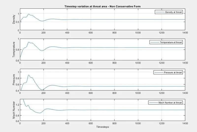
Time steps variation of the primitive variable at Throat area

Non Conservative Form

Conservative Form

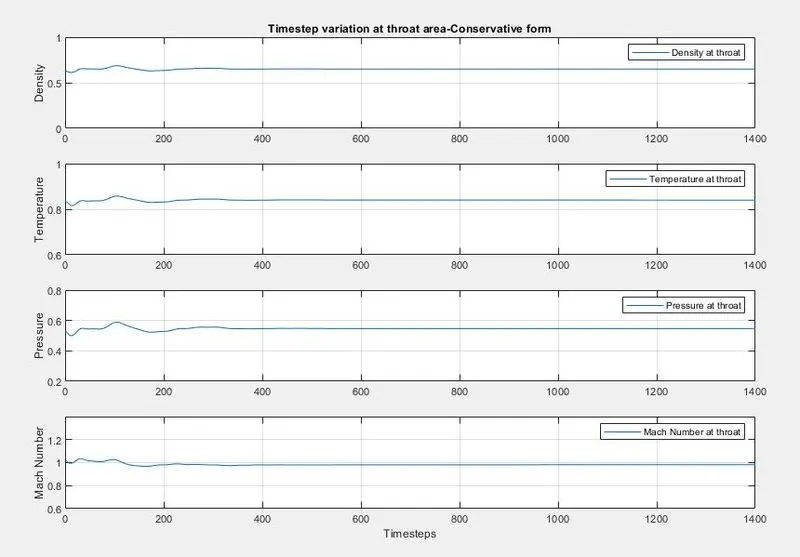
From the above plots, we can observe that due to initial variations time taken to be stable are more in the Non-Conservative form when compared to Conservative Form.

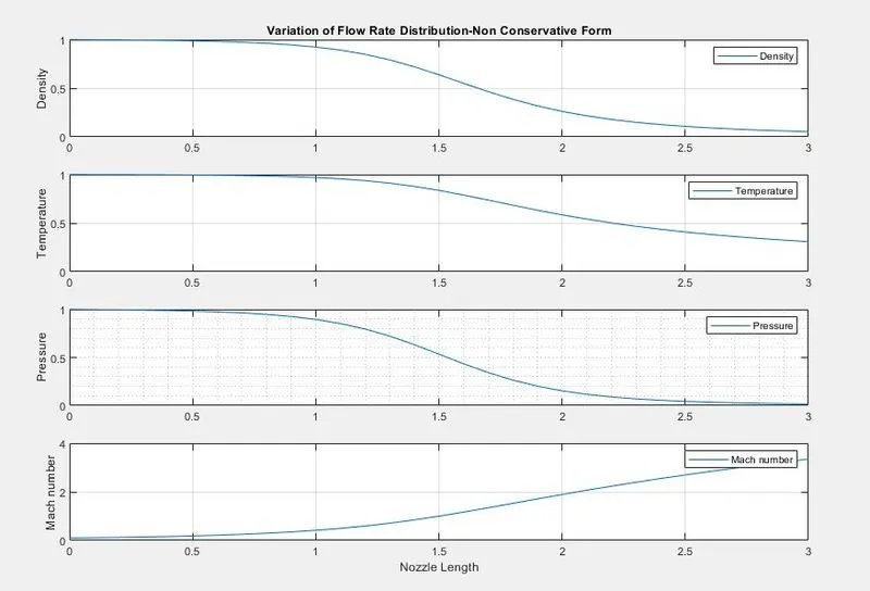
Variation of Flow Rate Distribution

Non Conservative Form

Conservative Form

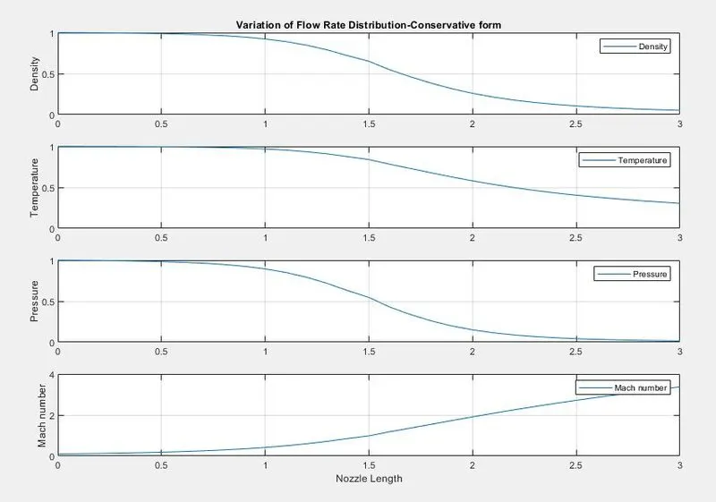
From the above plots, we can observe that for both Non-Conservative and Conservative forms graphs are the same as they have the same solution.

Mass flow rates at different Timesteps

Non Conservative form

Conservative Form

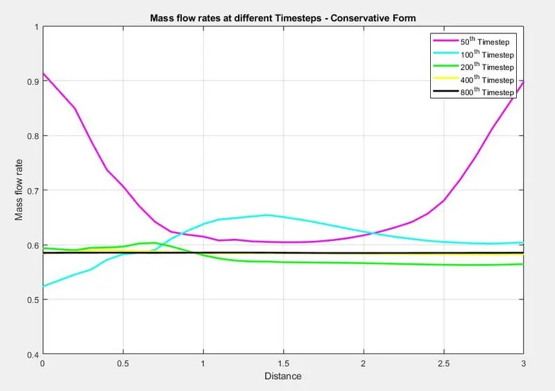
From above both plots we can observe that as the number of steps increases mass flow rate becomes stable.

Comparison Plot of Normalized Mass Flow Rate of both Non-Conservative Form & Conservative Form

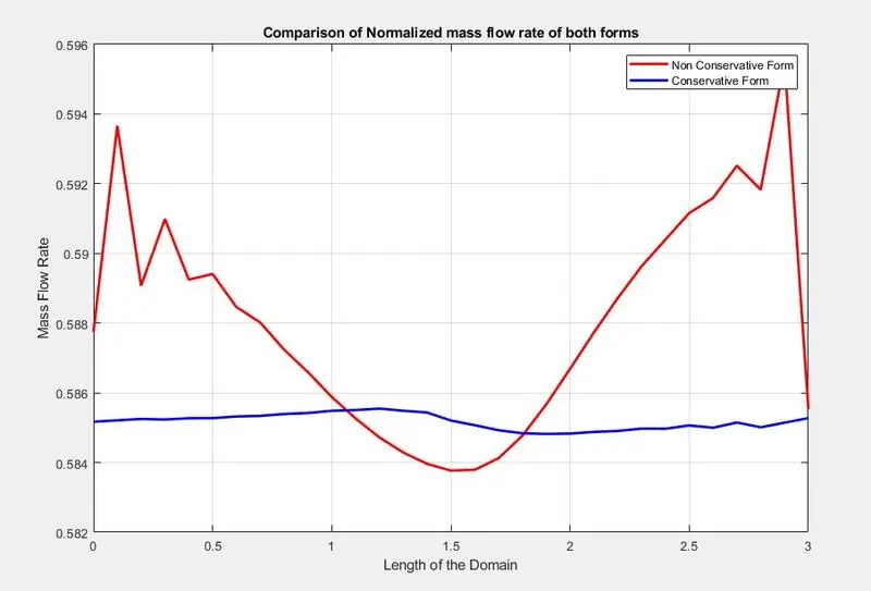
From the above plots, we can observe that the Conservative form attains stability in a lesser number of iterations.

The non-Conservative form oscillates much when compared to the Conservative form. The Conservative form gives an almost stable solution along the length.

Grid Independence Test

The mass flow rate variation in the nozzle for different grid numbers

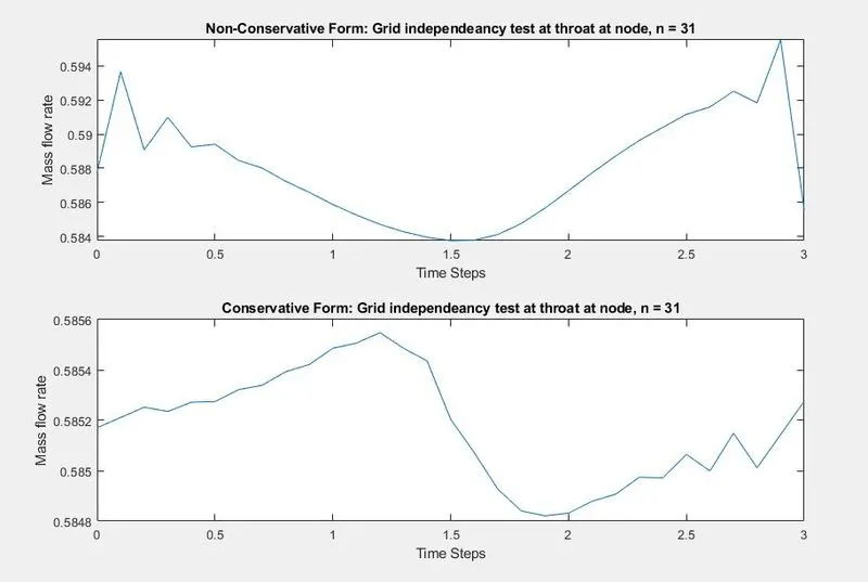
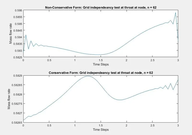
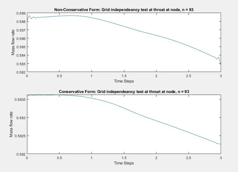
From the above plots, we can observe that there is a slight change at the throat area alone in the conservative form, which is not considered significant.