Week 5.1 - Mid term project - Solving the steady and unsteady 2D heat conduction problem
Aim:
To solve the Steady and Transient state 2D Heat Conduction Equation by using the point iteration techniques for both implicit and explicit schemes.
- Jacobi
- Gauss-Seidel
- Successive Over Relaxation
Theory:
The heat equation is a partial differencial equation that describes how the heat is distributed over time in a solid.
The three dimensional temperature heat conduction equation has both time and spatial derivative.
`(delT)/(delt) + alpha((del^2T)/(delx^2) + (del^2T)/(dely^2) + (del^2T)/(delz^2)) = 0`
here, `alpha` is thermal diffusivity.
This equation can be solved in two ways:
1. Steady-State Condition:
In this condition, the rate of change of temperature wrt time is equal to zero.
So, the 2D Steady-state heat equation becomes,
`(del^2T)/(delx^2) + (del^2T)/(dely^2) = 0`
2. Transient State Condition:
In this condition, both terms are considered,
So, the 2D Transient state heat equation becomes,
`(delT)/(delt) + alpha((del^2T)/(delx^2) + (del^2T)/(dely^2)) = 0`
Now, equations (a) and (b), will be solved by using iterative methods, in 2 different ways.
1. Explicit Method
2. Implicit Method
Note: We will use both these methods to solve the transient state equation.
Assumptions:
- The domain is a unit square.
- nx = ny [Number of points along the x-direction is equal to the number of points along the y-direction.]
- Tolerence = 1e-4
- Strating error = 9e-9
- The Boundary conditions are:
- Top Boundary = 600 K
- Bottom Boundary = 900 K
- Left Boundary = 400 K
- Right Boundary = 800 K
- Your absolute error criteria is 1e-4
A. Solving the steady state equation
`(del^2T)/(delx^2) + (del^2T)/(dely^2) = 0`
`T_p = (1/K){((T_L + T_R)/(Deltax^2)) + ((T_T + T_B)/(Deltay^2))}`
`T(i, j) = (1/K){((T_(old)(i-1, j) + T_(old)(i+1, j))/(dx^2)) + ((T_(old)(i, j-1) + T_(old)(i, j+1))/(dy^2))}`
`K = 2*(dx^2 + dy^2)/(dx^2 * dy^2)`
MATLAB Code for solving the equation using 3 iterative methods
Using Jacobi Iteration
% Solving the steady-state equation by using
% Jacobi Method

clear all
close all
clc

% Inputs
% nx = number of grids
nx = 10;
ny = nx;
% Domain length
l = 1;
x = linspace(0, l, nx)
y = linspace(0, l, ny)
dx = x(2) - x(1)
dy = y(2) - y(1)

% Tolerance error, start error
tol = 1e-4;
error = 9e9;
k = 2*((dx^2 + dy^2)/(dx^2 * dy^2));

% Boundary conditions
T_L = 400;
T_R = 800;
T_T = 600;
T_B = 900;

T(2:ny-1, 1) = T_L;
T(2:ny-1, nx) = T_R;
T(1, 2:nx-1) = T_T;
T(ny, 2:nx-1) = T_B;

% Average temperature at corners
T(1,1) = (T_T + T_L)/2;
T(nx,ny) = (T_R + T_B)/2;
T(1,ny) = (T_T + T_R)/2;
T(nx,1) = (T_L + T_B)/2;

T_initial = T;
Told = T;
% solving
iterative_solver = 1;
if iterative_solver == 1
    jacobi_iter_value = 1;

while(error > tol)
    for i=2:nx-1
        for j=2:ny-1
            term1 = (Told(i-1,j) + Told(i+1,j))/(k*(dx^2));
            term2 = (Told(i,j-1) + Told(i,j+1))/(k*(dy^2));
            T(i,j) = term1 + term2;
        end
    end


    error = max(max(abs(Told -T)));
    Told = T;
    jacobi_iter_value = jacobi_iter_value +1;


end
end
% Plotting
figure(1)
contourf(x, y, T)
clabel(contourf(x, y, T))
colormap(jet)
colorbar
set(gca, 'ydir', 'reverse')
title_text = sprintf('Jacobi iteration number for steady state = %d', jacobi_iter_value);
title(title_text)
xlabel('X axis')
ylabel('Y axis')
fprintf(' Number of Iterations for Jacobi Method for Steady state condition = %d', jacobi_iter_value)
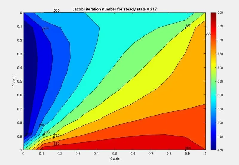
Graph:
Using Gauss-Seidel Iteration
% Solving the steady-state equation by using
% Gauss Seidel

clear all
close all
clc

% Inputs
% nx = number of grids
nx = 10;
ny = nx;
% Domain length
l = 1;
x = linspace(0, l, nx)
y = linspace(0, l, ny)
dx = x(2) - x(1)
dy = y(2) - y(1)

% Tolerance error, start error
tol = 1e-4;
error = 9e9;
k = 2*((dx^2 + dy^2)/(dx^2 * dy^2));

% Boundary conditions
T_L = 400;
T_R = 800;
T_T = 600;
T_B = 900;

T(2:ny-1, 1) = T_L;
T(2:ny-1, nx) = T_R;
T(1, 2:nx-1) = T_T;
T(ny, 2:nx-1) = T_B;

% Average temperature at corners
T(1,1) = (T_T + T_L)/2;
T(nx,ny) = (T_R + T_B)/2;
T(1,ny) = (T_T + T_R)/2;
T(nx,1) = (T_L + T_B)/2;

T_initial = T;
Told = T;
% solving
iterative_solver = 2;
if iterative_solver == 2
    gauss_iter_value = 1;

while(error > tol)
    for i=2:nx-1
        for j=2:ny-1
            term1 = (T(i-1,j) + Told(i+1,j))/(k*(dx^2));
            term2 = (T(i,j-1) + Told(i,j+1))/(k*(dy^2));
            T(i,j) = term1 + term2;
        end
    end


    error = max(max(abs(Told -T)));
    Told = T;
    gauss_iter_value = gauss_iter_value +1;


end
end
% Plotting
figure(1)
contourf(x, y, T)
clabel(contourf(x, y, T))
colormap(jet)
colorbar
set(gca, 'ydir', 'reverse')
title_text = sprintf('Gauss seidel iteration number for steady state = %d', gauss_iter_value);
title(title_text)
xlabel('X axis')
ylabel('Y axis')
fprintf(' Number of Iterations for Gauss Seidel Method for Steady state condition = %d', gauss_iter_value)
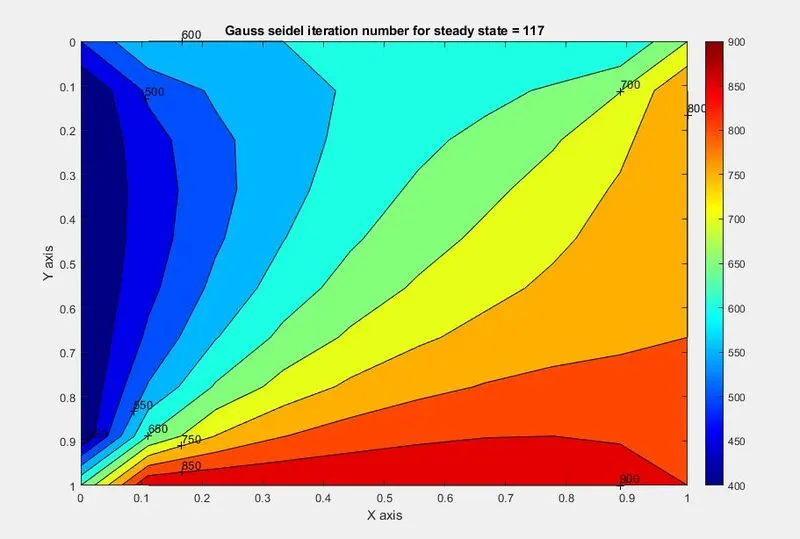
Graph:
Successive Over Relaxation Iteration
% Solving the steady-state equation by using
% successive over-relaxation method

clear all
close all
clc

% Inputs
% nx = number of grids
nx = 10;
ny = nx;
% Domain length
l = 1;
x = linspace(0, l, nx)
y = linspace(0, l, ny)
dx = x(2) - x(1)
dy = y(2) - y(1)

% Tolerance error, start error
tol = 1e-4;
error = 9e9;
omega = 1.2;
k = 2*((dx^2 + dy^2)/(dx^2 * dy^2));

% Boundary conditions
T_L = 400;
T_R = 800;
T_T = 600;
T_B = 900;

T(2:ny-1, 1) = T_L;
T(2:ny-1, nx) = T_R;
T(1, 2:nx-1) = T_T;
T(ny, 2:nx-1) = T_B;

T(1,1) = (T_T + T_L)/2;
T(nx,ny) = (T_R + T_B)/2;
T(1,ny) = (T_T + T_R)/2;
T(nx,1) = (T_L + T_B)/2;

T_initial = T;
Told = T;
% solving
iterative_solver = 3;
if iterative_solver == 3
    sor_iter_value = 1;

while(error > tol)
    for i=2:nx-1
        for j=2:ny-1
            term1 = (T(i-1,j) + Told(i+1,j))/(k*(dx^2));
            term2 = (T(i,j-1) + Told(i,j+1))/(k*(dy^2));
            T(i,j) = omega*(term1 + term2)+ (1-omega)*Told(i,j);
        end
    end


    error = max(max(abs(Told -T)));
    Told = T;
    sor_iter_value = sor_iter_value +1;


end
end
% Plotting
figure(1)
contourf(x, y, T)
clabel(contourf(x, y, T))
colormap(jet)
colorbar
set(gca, 'ydir', 'reverse')
title_text = sprintf('SOR iteration number for steady state = %d', sor_iter_value);
title(title_text)
xlabel('X axis')
ylabel('Y axis')
fprintf(' Number of Iterations for SOR Method for Steady state condition = %d', sor_iter_value)
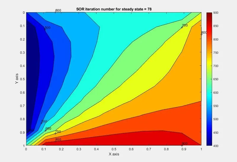
Graph:
B. Solving the Transient state equation
Using Implicit Scheme
`(delT)/(delt)+alpha((del^2T)/(delx^2) + (del^2T)/(dely^2)) = 0`
`T_(P)^(n+1) = T_(P)^(n) + (alphaDeltat)((T_R-2T_P+T_L)/(Deltax^2) + (T_T-2T_P+T_B)/(Deltay^2))`
`T_P^(n+1) = (1/(1+2k1+2k2))(T_P^(n) + k1(T_L^(n+1) + T_R^(n+1)) + k2(T_T^(n+1) + T_B^(n+1)))`
`k1 = alpha((Deltat)/(Deltax^2)), k2 = alpha((Deltat)/(Deltay^2))`
`T_(i, j) = (1/(1+2k1+2k2))(T_(i,j) + k1(T_(i-1, j) + T_(i+1, j)) + k2(T_(i, j-1) + T_(i, j+1)))`
MATLAB Code for solving the equation using 3 iterative methods
Using Jacobi Iteration
% Solving the steady-state equation by using
% Jacobi method
% Implicit Method

clear all
close all
clc

% Inputs
% nx = number of grids
nx = 10;
ny = nx;
nt = 1400;
% Domain length
l = 1;
x = linspace(0, l, nx)
y = linspace(0, l, ny)
dx = x(2) - x(1)
dy = y(2) - y(1)

% Tolerance error, start error
tol = 1e-4;
error = 9e9;
dt = 1e-3;
alpha = 1.4
k1 = alpha*(dt/(dx^2));
k2 = alpha*(dt/(dy^2));

% Boundary conditions
T_L = 400;
T_R = 800;
T_T = 600;
T_B = 900;

T = 300*ones(nx,ny);

T(2:ny-1, 1) = T_L;
T(2:ny-1, nx) = T_R;
T(1, 2:nx-1) = T_T;
T(ny, 2:nx-1) = T_B;

T(1,1) = (T_T + T_L)/2;
T(nx,ny) = (T_R + T_B)/2;
T(1,ny) = (T_T + T_R)/2;
T(nx,1) = (T_L + T_B)/2;

T_initial = T;
Told = T;
% solving
jacobi_iter_value = 1;
for k = 1:nt
    error = 9e9;

    while(error > tol)
        for i=2:nx-1
            for j=2:ny-1
                term1 = 1/(1 + (2*k1) + (2*k2));
                term2 = k1*term1;
                term3 = k2*term1;
                H = (Told(i-1,j) + Told(i+1,j));
                V = (Told(i,j-1) + Told(i,j+1));
                T(i,j) = (T_initial(i,j)*term1) + H*(term2) + V*(term3);
            end
        end

        error = max(max(abs(Told -T)));
        Told = T;
        jacobi_iter_value = jacobi_iter_value +1;


    end
    % Plotting
    T_initial = T
    figure(1)
    contourf(x, y, T)
    clabel(contourf(x, y, T))
    colormap(jet)
    colorbar
    set(gca, 'ydir', 'reverse')
    title_text = sprintf('Jacobi iteration number for unsteady state = %d', jacobi_iter_value);
    title(title_text)
    xlabel('X axis')
    ylabel('Y axis')
end

fprintf(' Number of Iterations for Implicit Jacobi Method for Transient State Condition = %d', jacobi_iter_value)
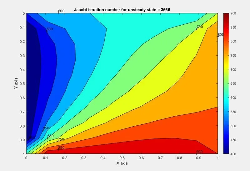
Graph:
Using Gauss-Seidel Iteration
% Solving the steady-state equation by using
% Gauss-Seidel method
% Implicit Method

clear all
close all
clc

% Inputs
% nx = number of grids
nx = 10;
ny = nx;
nt = 1400;
% Domain length
l = 1;
x = linspace(0, l, nx)
y = linspace(0, l, ny)
dx = x(2) - x(1)
dy = y(2) - y(1)

% Tolerance error, start error
tol = 1e-4;
error = 9e9;
dt = 1e-3;
alpha = 1.4

k1 = alpha*(dt/(dx^2));
k2 = alpha*(dt/(dy^2));

% Boundary conditions
T_L = 400;
T_R = 800;
T_T = 600;
T_B = 900;

T = 300*ones(nx,ny);

T(2:ny-1, 1) = T_L;
T(2:ny-1, nx) = T_R;
T(1, 2:nx-1) = T_T;
T(ny, 2:nx-1) = T_B;

T(1,1) = (T_T + T_L)/2;
T(nx,ny) = (T_R + T_B)/2;
T(1,ny) = (T_T + T_R)/2;
T(nx,1) = (T_L + T_B)/2;

T_initial = T;
Told = T;
% solving
Gauss_iter_value = 1;
for k = 1:nt
    error = 9e9;

    while(error > tol)
        for i=2:nx-1
            for j=2:ny-1
                term1 = 1/(1 + (2*k1) + (2*k2));
                term2 = k1*term1;
                term3 = k2*term1;
                H = (T(i-1,j) + Told(i+1,j));
                V = (T(i,j-1) + Told(i,j+1));
                T(i,j) = (T_initial(i,j)*term1) + H*(term2) + V*(term3);
            end
        end

        error = max(max(abs(Told -T)));
        Told = T;
        Gauss_iter_value = Gauss_iter_value +1;


    end
    % Plotting
    T_initial = T
    figure(1)
    contourf(x, y, T)
    clabel(contourf(x, y, T))
    colormap(jet)
    colorbar
    set(gca, 'ydir', 'reverse')
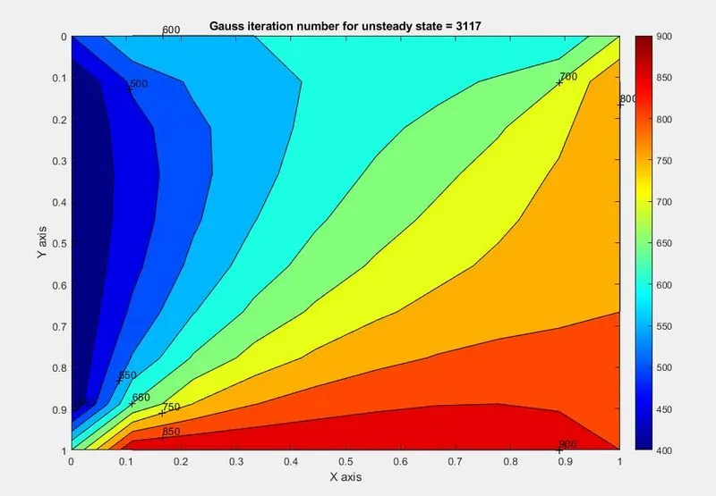
    title_text = sprintf('Gauss iteration number for unsteady state = %d', Gauss_iter_value);
    title(title_text)
    xlabel('X axis')
    ylabel('Y axis')
end

fprintf(' Number of Iterations for Implicit Gauss Seidel Method for Transient State Condition = %d', Gauss_iter_value)
Graph:
Successive Over Relaxation Iteration
% Solving the steady-state equation by using
% Successive Over-Relaxation method
% Implicit Method

clear all
close all
clc

% Inputs
% nx = number of grids
nx = 10;
ny = nx;
nt = 1400;
% Domain length
l = 1;
x = linspace(0, l, nx)
y = linspace(0, l, ny)
dx = x(2) - x(1)
dy = y(2) - y(1)

% Tolerance error, start error
tol = 1e-4;
error = 9e9;
dt = 1e-3;
omega = 1.2
alpha = 1.4;

k1 = alpha*(dt/(dx^2));
k2 = alpha*(dt/(dy^2));

% Boundary conditions
T_L = 400;
T_R = 800;
T_T = 600;
T_B = 900;

T = 300*ones(nx,ny);

T(2:ny-1, 1) = T_L;
T(2:ny-1, nx) = T_R;
T(1, 2:nx-1) = T_T;
T(ny, 2:nx-1) = T_B;

T(1,1) = (T_T + T_L)/2;
T(nx,ny) = (T_R + T_B)/2;
T(1,ny) = (T_T + T_R)/2;
T(nx,1) = (T_L + T_B)/2;

T_initial = T;
Told = T;
T_end = T

% solving
SOR_iter_value = 1;
for k = 1:nt
    error = 9e9;

    while(error > tol)
        for i=2:nx-1
            for j=2:ny-1
                term1 = 1/(1 + (2*k1) + (2*k2));
                term2 = k1*term1;
                term3 = k2*term1;
                H = (T(i-1,j) + Told(i+1,j));
                V = (T(i,j-1) + Told(i,j+1));
                T(i,j) = (T_initial(i,j)*term1) + H*(term2) + V*(term3);
                T_end(i,j) = ((1-omega)*Told(i,j))+ (T(i,j)*omega);
            end
        end

        error = max(max(abs(Told -T)));
        Told = T_end;
        SOR_iter_value = SOR_iter_value +1;


    end
    % Plotting
    T_initial = T
    figure(1)
    contourf(x, y, T)
    clabel(contourf(x, y, T))
    colormap(jet)
    colorbar
    set(gca, 'ydir', 'reverse')
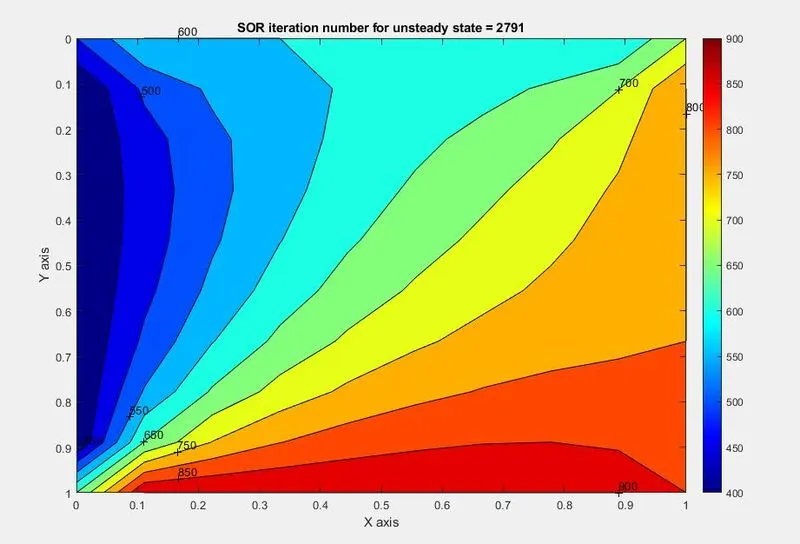
    title_text = sprintf('SOR iteration number for unsteady state = %d', SOR_iter_value);
    title(title_text)
    xlabel('X axis')
    ylabel('Y axis')
end

fprintf(' Number of Iterations for Implicit SOR Method for Transient State Condition = %d', SOR_iter_value)
Graph:
Using Explicit Scheme
`(delT)/(delt)+alpha((del^2T)/(delx^2) + (del^2T)/(dely^2)) = 0`
`T_(P)^(n+1) = T_(P)^(n) + (alphaDeltat)((T_R-2T_P+T_L)/(Deltax^2) + (T_T-2T_P+T_B)/(Deltay^2))`
`T_p^(n+1) = (T_p^(n) + k1(T_L^(n) -2T_P^(n)+ T_R^(n)) + k2(T_T^(n) -2T_P^(n)+ T_B^(n)))`
`k1 = alpha((Deltat)/(Deltax^2)), k2 = alpha((Deltat)/(Deltay^2))`
`T_(i, j) = (T_(i,j) + k1(T_(i-1, j)-2T_(i,j) + T_(i+1, j)) + k2(T_(i, j-1)-2T_(i,j) + T_(i, j+1)))`
MATLAB Code for solving the equation
Using Jacobi Iteration
% Solving the steady-state equation by using
% Jacobi method
% Explicit scheme

clear all
close all
clc

% Inputs
% nx = number of grids
nx = 10;
ny = nx;
nt = 1400;
% Domain length
l = 1;
x = linspace(0, l, nx)
y = linspace(0, l, ny)
dx = x(2) - x(1)
dy = y(2) - y(1)

% Tolerance error, start error
tol = 1e-4;
error = 9e9;
dt = 1e-3;
alpha = 1.4

k1 = alpha*(dt/(dx^2));
k2 = alpha*(dt/(dy^2));

% Boundary conditions
T_L = 400;
T_R = 800;
T_T = 600;
T_B = 900;

T = 300*ones(nx,ny);

T(2:ny-1, 1) = T_L;
T(2:ny-1, nx) = T_R;
T(1, 2:nx-1) = T_T;
T(ny, 2:nx-1) = T_B;

T(1,1) = (T_T + T_L)/2;
T(nx,ny) = (T_R + T_B)/2;
T(1,ny) = (T_T + T_R)/2;
T(nx,1) = (T_L + T_B)/2;

T_initial = T;
Told = T;
% solving
jacobi_iter_value = 1;
for k = 1:nt
    error = 9e9;

    while(error > tol)
        for i=2:nx-1
            for j=2:ny-1
                term1 = Told(i,j);
                term2 = k1*(Told(i-1,j) - 2*Told(i,j) + Told(i+1,j));
                term3 = k2*(Told(i,j-1) - 2*Told(i,j) + Told(i,j+1));
                T(i,j) = term1 + term2 + term3;
            end
        end

        error = max(max(abs(Told -T)));
        Told = T;
        jacobi_iter_value = jacobi_iter_value +1;


    end
    % Plotting
    figure(1)
    contourf(x, y, T)
    clabel(contourf(x, y, T))
    colormap(jet)
    colorbar
    set(gca, 'ydir', 'reverse')
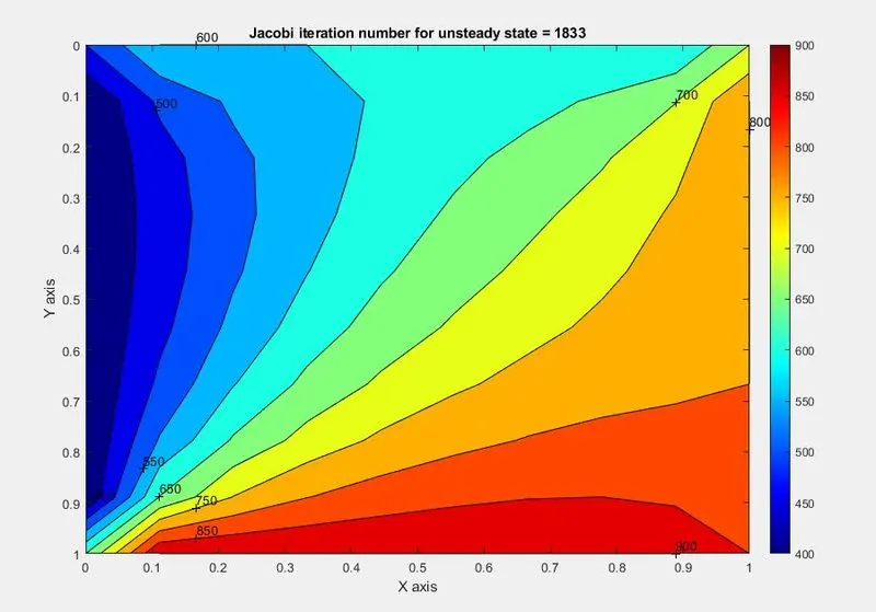
    title_text = sprintf('Jacobi iteration number for unsteady state = %d', jacobi_iter_value);
    title(title_text)
    xlabel('X axis')
    ylabel('Y axis')
end

fprintf(' Number of Iterations for Explicit Jacobi for Transient method = %d', jacobi_iter_value)
Graph:
Conclusion:
| Type of scheme | Methods used | No. of Iterations |
| Implicit Steady State |
1. Jacobi 2. Gauss Seidel 3. SOR |
1. 217 2. 117 3. 78 |
| Implicit Transient State |
1. Jacobi 2. Gauss Seidel 3. SOR |
1. 3666 2. 3117 3. 2791 |
| Explicit Transient State | 1. Jacobi | 1. 1833 |
- In the Steady-state equation, the SOR method takes the least number of iteration for solving the equation.
- In the case of Transient equations, the time required to solve the equation is more when compared to the steady-state condition in solving the problem.
- In Transient state cases, explicit methods take less time than implicit methods.