Week 3.5 - Deriving 4th order approximation of a 2nd order derivative using Taylor Table method

In this exercise, we will derive the following 4^th order approximation of the second-order derivative

1. Central difference
2. Skewed right-sided difference
3. Skewed left-sided difference

Derivation of the 4^th order approximation of the second-order derivative:

1. Using the Central Difference Scheme:

Total number of Nodes, N = 5

Order of derivative, Q = 2

Order of accuracy, P = N-Q+1 = 5-2+1

P = 4 ........(i)

For central difference scheme, numerical stencil looks like:

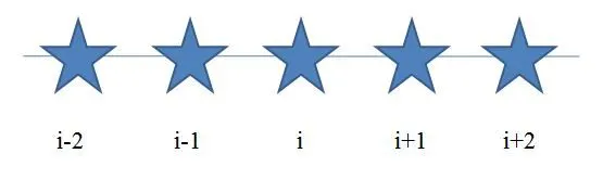
In this case, to compute the 4^th order approximation at point (i), we will take information from the points (i-2), (i-1), (i+1), and (i+2).

From the above points, we start with this equation:

`(del^2u)/(delx^2) = af(i-2) +bf(i-1) + cf(i) +df(i+1) +ef(i+2)` .........(1)

Now, to find the values (a, b, c, d, e), we will use the Taylor Table method. Also, we write each term of equation (1) as:

`af(i-2) = a[f(i) - ((2Deltax)f^'(i))/(1!) + ((2Deltax)^2f^('')(i))/(2!) - ((2Deltax)^3f^(''')(i))/(3!) + ((2Deltax)^4f^('''')(i))/(4!) - ((2Deltax)^5f^(''''') (i))/(5!) + ......]`

`bf(i-1) = b[f(i) - ((Deltax)f^'(i))/(1!) + ((Deltax)^2f^('')(i))/(2!) - ((Deltax)^3f^(''')(i))/(3!) + ((Deltax)^4f^('''')(i))/(4!) - ((Deltax)^5f^(''''') (i))/(5!) + ......]`

`cf(i) = cf(i)`

`df(i+1) = d[f(i) + ((Deltax)f^'(i))/(1!) + ((Deltax)^2f^('')(i))/(2!) + ((Deltax)^3f^(''')(i))/(3!) + ((Deltax)^4f^('''')(i))/(4!) + ((Deltax)^5f^(''''') (i))/(5!) + ......]`

`ef(i+2) = e[f(i) + ((2Deltax)f^'(i))/(1!) + ((2Deltax)^2f^('')(i))/(2!) + ((2Deltax)^3f^(''')(i))/(3!) + ((2Deltax)^4f^('''')(i))/(4!) + ((2Deltax)^5f^(''''') (i))/(5!) + ......]`

Arranging the above Taylor series expansion in Table, we get

Note: To get this table, we take one row, then take its coefficient term for the first column, from the second column onwards we multiple previous column term by:

(the numerical value from terms ((i-2), (i-1), etc.) at which we are writing Taylor series)/(power of `Deltax`).

	`f(i)`	`Deltaxf^(')(i)`	`(Deltax)^2f^('')(i)`	`(Deltax)^3f^(''')(i)`	`(Deltax)^4f^('''')(i)`	`(Deltax)^5f^(''''')(i)`	`(Deltax)^6f^('''''')(i)`
`af(i-2)`	`a`	`-2a`	`(4a)/2`	`(-8a)/6`	`(16a)/24`	`-(32a)/120`	`(64a)/720`
`bf(i-1)`	`b`	`-b`	`b/2`	`(-b)/6`	`b/24`	`(-b)/120`	`b/720`
`cf(i)`	`c`	0	0	0	0	0	0
`df(i+1)`	`d`	`d`	`d/2`	`d/6`	`d/24`	`(d)/120`	`d/720`
`ef(i+2)`	`e`	`2e`	`(4e)/2`	`(8e)/6`	`(16e)/24`	`(32e)/120`	`(64e)/720`
`sum(af(i-2) + bf(i-1) + cf(i) + df(i+1) + ef(i+2))`	0	0	1	0	0	?	?

Note: As the above expansion is till 5 terms, so up to 5 terms we get sum. After that sum will be unknown.

Now, we have 5 unknowns and we get 5 equations.

`a + b + c + d + e = 0` ....(2)

`-2a - b + 0 + d + 2e = 0` ....(3)

`2a + b/2 + 0 + d/2 + 2e = 1` ....(4)

`(-8a)/6 + (-b)/6 + 0 + d/6 + (8e)/6 = 0` ....(5)

`(16a)/24 + b/24 + 0 + d/24 + (16e)/24 = 0` ....(6)

We will solve above equations using Matrix Inversion Method.

AX = B

X = inv(A)*B

`[[1, 1, 1, 1, 1], [-2, -1, 0, 1, 2], [2, 1/2, 0, 1/2, 2], [-8/6, -1/6, 0, 1/6, 8/6], [16/24, 1/24, 0, 1/24, 16/24]] [[a], [b], [c], [d], [e]] = [[0], [0], [1], [0], [0]]`

We get coefficient as,

a = -0.0833, b = 1.333, c = -2.500, d = 1.333, e = -0.0833

Now, dividing the right side of equation (1) by (Deltax)^2) for putting the obtained values of (a, b, c, d, e), we get

`(del^2u)/(delx^2) = (af(i-2) + bf(i-1) + cf(i) + ef(i+1) + df(i+2)) /((Deltax)^2)` .......(A)

Now, putting these values in equation (A), we get

`(del^2u)/(delx^2) = ((-0.0833)f(i-2) + (1.333)f(i-1) + (-2.500)f(i) + (1.333)f(i+1) + (-0.0833)f(i+2)) /((Deltax)^2)`

From our Taylor Table:

`(del^2u)/(delx^2) = (a+b+c+d+e)f(i) + (-2a-b+0+d+2e)(Deltax)f^'(i) + (2a+b/2+0+d/2+2e)(Deltax)^2f^('')(i) + ((-8a)/6+(-b)/6+0+d/6+(8e)/6)(Deltax)^3f^(''')(i) + ((16a)/24+b/24+0+d/24+(16e)/24)(Deltax)^4f^('''')(i) + ((-32a)/120+(-b)/120+0+d/120+(32e)/120)(Deltax)^5f^(''''') (i) + ((64a)/720+(b)/720+0+d/720+(64e)/720)(Deltax)^6f^('''''') (i)` ....(B)

Putting values from equations (2), (3), (4), (5), (6) into equation (B),

Note: First, second, fourth, and fifth terms are zero; we get the third term is 1; also on rearrangement we get the sixth term equal to zero.

`(del^2u)/(delx^2) = (2a+b/2+0+d/2+2e)(Deltax)^2f^('')(i) + ((64a)/720+(b)/720+0+d/720+(64e)/720)(Deltax)^6f^('''''') (i)`

On dividing above equation by `(Deltax)^2`, we get

`(del^2u)/(delx^2) = (2a+b/2+0+d/2+2e)f^('')(i) + ((64a)/720+(b)/720+0+d/720+(64e)/720)(Deltax)^4f^('''') (i)`

The term with `(Deltax)^4` denotes truncation error.

So, the order of the truncation error `O(Deltax^4)` is 4.

Also, from equation (i), we can verify this.

Finally, the equation is:

`(del^2u)/(delx^2) = (2(-0.0833)+1.333/2+0+1.333/2+2(-0.0833))f^('')(i) + ((64(-0.0833))/720+(1.333)/720+0+1.333/720+(64(-0.0833))/720)(Deltax)^4f^('''''') (i)`

2. Using the Skewed Right-Sided Difference Scheme:

Total number of Nodes, N = 6

Order of derivative, Q = 2

Order of accuracy, P = N-Q = 6-2

P = 4 ........(i)

For skewed right-sided difference scheme, numerical stencil looks like this:

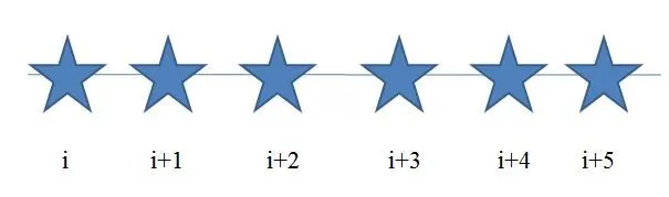
In this case, to compute the 4^th order approximation at point (i), we will take information from the points (i+1), (i+2), (i+3), (i+4), and (i+5).

From the above points, we start with this equation:

`(del^2u)/(delx^2) = af(i) +bf(i+1) + cf(i+2) +df(i+3) +ef(i+4) + gf(i+5)` ....(1)

Now, to find the values (a, b, c, d, e, f), we will use the Taylor Table method. Also, we write each term of equation (1) as:

`af(i) = af(i)`

`bf(i+1) = b[f(i) + ((Deltax)f^'(i))/(1!) + ((Deltax)^2f^('')(i))/(2!) + ((Deltax)^3f^(''')(i))/(3!) + ((Deltax)^4f^('''')(i))/(4!) + ((Deltax)^5f^(''''') (i))/(5!) + ((Deltax)^6f^('''''') (i))/(6!) + ......]`

`cf(i+2) = c[f(i) + ((2Deltax)f^'(i))/(1!) + ((2Deltax)^2f^('')(i))/(2!) + ((2Deltax)^3f^(''')(i))/(3!) + ((2Deltax)^4f^('''')(i))/(4!) + ((2Deltax)^5f^(''''') (i))/(5!) + ((2Deltax)^6f^('''''') (i))/(6!) + ......]`

`df(i+3) = d[f(i) + ((3Deltax)f^'(i))/(1!) + ((3Deltax)^2f^('')(i))/(2!) + ((3Deltax)^3f^(''')(i))/(3!) + ((3Deltax)^4f^('''')(i))/(4!) + ((3Deltax)^5f^(''''') (i))/(5!) + ((3Deltax)^6f^('''''') (i))/(6!) + ......]`

`ef(i+4) = e[f(i) + ((4Deltax)f^'(i))/(1!) + ((4Deltax)^2f^('')(i))/(2!) + ((4Deltax)^3f^(''')(i))/(3!) + ((4Deltax)^4f^('''')(i))/(4!) + ((4Deltax)^5f^(''''') (i))/(5!) + ((4Deltax)^6f^('''''') (i))/(6!) + ......]`

`gf(i+5) = g[f(i) + ((5Deltax)f^'(i))/(1!) + ((5Deltax)^2f^('')(i))/(2!) + ((5Deltax)^3f^(''')(i))/(3!) + ((5Deltax)^4f^('''')(i))/(4!) + ((5Deltax)^5f^(''''') (i))/(5!) + ((5Deltax)^6f^('''''') (i))/(6!) + ......]`

Arranging the above Taylor series expansion in Table, we get

Note: To get this table, we take one row, then take its coefficient term for the first column, from the second column onwards we multiple previous column term by:

(the numerical value from terms ((i+1), (i+2), etc.) at which we are writing Taylor series)/(power of `Deltax`).

	`f(i)`	`Deltaxf^(')(i)`	`(Deltax)^2f^('')(i)`	`(Deltax)^3f^(''')(i)`	`(Deltax)^4f^('''')(i)`	`(Deltax)^5f^(''''')(i)`	`(Deltax)^6f^('''''')(i)`
`af(i)`	`a`	0	0	0	0	0	0
`bf(i+1)`	`b`	`b`	`b/2`	`(b)/6`	`b/24`	`(b)/120`	`b/720`
`cf(i+2)`	`c`	`2c`	`(4c)/2`	`(8c)/6`	`(16c)/24`	`(32c)/120`	`(64c)/720`
`df(i+3)`	`d`	`3d`	`(9d)/2`	`(27d)/6`	`(81d)/24`	`(243d)/120`	`(729d)/720`
`ef(i+4)`	`e`	`4e`	`(16e)/2`	`(64e)/6`	`(256e)/24`	`(1024e)/120`	`(4096e)/720`
`gf(i+5)`	`g`	`5g`	`(25g)/2`	`(125g)/6`	`(625g)/24`	`(3125g)/120`	`(15625g)/720`
`sum(af(i) + bf(i+1) + cf(i+2) + df(i+3) + ef(i+4) + gf(i+5))`	0	0	1	0	0	0	?

Note: As the above expansion is till 6 terms, so up to 6 terms we get sum. After that sum will be unknown.

Now, we have 6 unknowns and we get 6 equations.

`a + b + c + d + e + g = 0` ....(2)

`0 + b + 2c + 3d + 4e + 5g = 0` ....(3)

`0 + b/2 + 2c + (9d)/2 + 8e + (25g)/2 = 1` ....(4)

`0 + (b)/6 + (8c)/6 + (27d)/6 + (64e)/6 + (125g)/6 = 0` ....(5)

`0 + b/24 + (16c)/24 + (81d)/24 + (256e)/24 + (625g)/24 = 0` ....(6)

`0 + b/120 + (32c)/120 + (243d)/120 + (1024e)/120 + (3125g)/120 = 0` ....(7)

We will solve above equations using Matrix Inversion Method.

AX = B

X = inv(A)*B

`[[1, 1, 1, 1, 1, 1], [0, 1, 2, 3, 4, 5], [0, 1/2, 2, 9/2, 8, 25/2], [0, 1/6, 8/6, 27/6, 64/6, 125/6], [0, 1/24, 16/24, 81/24, 256/24, 1024/24], [0, 1/120, 32/120, 243/120, 1024/120, 3125/120]] [[a], [b], [c], [d], [e], [g]] = [[0], [0], [1], [0], [0], [0]]`

We get coefficient as,

a = 3.7500, b = -12.833, c = 17.833, d = -13.000, e = 5.0833, g = -0.833

Now, dividing the right side of equation (1) (Deltax)^2) to put the obtained values of (a, b, c, d, e, g), we get

`(del^2u)/(delx^2) = (af(i) +bf(i+1) + cf(i+2) +df(i+3) +ef(i+4) + gf(i+5)) /((Deltax)^2)` .......(A)

Now, putting these values in equation (A), we get

`(del^2u)/(delx^2) = ((3.7500)f(i) +(-12.833)f(i+1) + (17.833)f(i+2) +(-13.000)f(i+3) +(5.0833)f(i+4) + (-0.833)f(i+5)) /((Deltax)^2)`

From our Taylor Table:

`(del^2u)/(delx^2) = (a+b+c+d+e)f(i) + (0 + b + 2c + 3d + 4e + 5g)(Deltax)f^'(i) + (0 + b/2 + 2c + (9d)/2 + 8e + (25g)/2)(Deltax)^2f^('')(i) + (0 + (b)/6 + (8a)/6 + (27d)/6 + (64e)/6 + (125g)/6)(Deltax)^3f^(''')(i) + (0 + b/24 + (16c)/24 + (81d)/24 + (256e)/24 (625g)/24)(Deltax)^4f^('''')(i) + (0 + b/120 + (32c)/120 + (243d)/120 + (1024e)/120 + (3125g)/120)(Deltax)^5f^(''''') (i) + (0+(b)/720+(64c)/720+(729d)/720+(4096e)/720+(15625g)/720)(Deltax)^6f^('''''') (i)` ....(B)

Putting values from equations (2), (3), (4), (5), (6), (7) into equation (B),

Note: First, second, fourth, fifth, and sixth terms are zero; we get the third term is 1.

`(del^2u)/(delx^2) = (0 + b/2 + 2c + (9d)/2 + 8e + (25g)/2)(Deltax)^2f^('')(i) + ((0+(b)/720+(64c)/720+(729d)/720+(4096e)/720+(15625g)/720)(Deltax)^6f^('''''') (i)`

On dividing above equation by `(Deltax)^2`, we get

`(del^2u)/(delx^2) = (0 + b/2 + 2c + (9d)/2 + 8e + (25g)/2)f^('')(i) + (0+(b)/720+(64c)/720+(729d)/720+(4096e)/720+(15625g)/720)(Deltax)^4f^('''') (i)`

The term with `(Deltax)^4` denotes truncation error.

So, the order of the truncation error `O(Deltax^4)` is 4.

Also, from equation (i), we can verify this.

Finally, the equation is:

`(del^2u)/(delx^2) = (0 + (-12.833)/2 + 2(17.833) + (9(-13.000))/2 + 8(5.0833) + (25(-0.833))/2)f^('')(i) + (0+(-12.833)/720+(64(17.833))/720+(729(-13.00))/720+(4096(5.0833))/720+(15625(-0.833))/720)(Deltax)^4f^('''')`

3. Using the Skewed Left-Sided Difference Scheme:

Total number of Nodes, N = 6

Order of derivative, Q = 2

Order of accuracy, P = N-Q = 6-2

P = 4 ........(i)

For skewed left-sided difference scheme, numerical stencil looks like this:

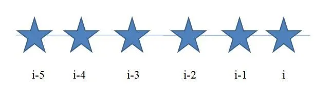
In this case, to compute the 4^th order approximation at point (i), we will take information from the points (i-5), (i-4), (i-3), (i-2), and (i-1).

From the above points, we start with this equation:

`(del^2u)/(delx^2) = af(i-5) +bf(i-4) + cf(i-3) +df(i-2) +ef(i-1) + gf(i)` ....(1)

Now, to find the values (a, b, c, d, e, f), we will use the Taylor Table method. Also, we write each term of equation (1) as:

`af(i-5) = a[f(i) - ((5Deltax)f^'(i))/(1!) + ((5Deltax)^2f^('')(i))/(2!) - ((5Deltax)^3f^(''')(i))/(3!) + ((5Deltax)^4f^('''')(i))/(4!) - ((5Deltax)^5f^(''''') (i))/(5!) + ((5Deltax)^6f^('''''') (i))/(6!) - ......]`

`bf(i-4) = b[f(i) - ((4Deltax)f^'(i))/(1!) + ((4Deltax)^2f^('')(i))/(2!) - ((4Deltax)^3f^(''')(i))/(3!) + ((4Deltax)^4f^('''')(i))/(4!) - ((4Deltax)^5f^(''''') (i))/(5!) + ((4Deltax)^6f^('''''') (i))/(6!) - ......]`

`cf(i-3) = c[f(i) - ((3Deltax)f^'(i))/(1!) + ((3Deltax)^2f^('')(i))/(2!) - ((3Deltax)^3f^(''')(i))/(3!) + ((3Deltax)^4f^('''')(i))/(4!) - ((3Deltax)^5f^(''''') (i))/(5!) + ((3Deltax)^6f^('''''') (i))/(6!) - ......]`

`df(i-2) = d[f(i) - ((2Deltax)f^'(i))/(1!) + ((2Deltax)^2f^('')(i))/(2!) - ((2Deltax)^3f^(''')(i))/(3!) + ((2Deltax)^4f^('''')(i))/(4!) - ((2Deltax)^5f^(''''') (i))/(5!) + ((2Deltax)^6f^('''''') (i))/(6!) - ......]`

`ef(i-1) = e[f(i) - ((Deltax)f^'(i))/(1!) + ((Deltax)^2f^('')(i))/(2!) - ((Deltax)^3f^(''')(i))/(3!) + ((Deltax)^4f^('''')(i))/(4!) - ((Deltax)^5f^(''''') (i))/(5!) + ((Deltax)^6f^('''''') (i))/(6!) - ......]`

`gf(i) = gf(i)`

Arranging the above Taylor series expansion in Table, we get

Note: To get this table, we take one row, then take its coefficient term for the first column, from the second column onwards we multiple previous column term by:

(the numerical value from terms ((i-1), (i-2), etc.) at which we are writing Taylor series)/(power of `Deltax`).

	`f(i)`	`Deltaxf^(')(i)`	`(Deltax)^2f^('')(i)`	`(Deltax)^3f^(''')(i)`	`(Deltax)^4f^('''')(i)`	`(Deltax)^5f^(''''')(i)`	`(Deltax)^6f^('''''')(i)`
`af(i-5)`	`a`	`-5a`	`(25a)/2`	`(-125a)/6`	`(625a)/24`	`(-3125a)/120`	`(15625a)/720`
`bf(i-4)`	`b`	`-4b`	`8b`	`(-64b)/6`	`(256b)/24`	`(-1024b)/120`	`(4096b)/720`
`cf(i-3)`	`c`	`-3c`	`(9c)/2`	`(-27c)/6`	`(81c)/24`	`(-243c)/120`	`(729c)/720`
`df(i-2)`	`d`	`-2d`	`2d`	`(-8d)/6`	`(16d)/24`	`(-32d)/120`	`(64d)/720`
`ef(i-1)`	`e`	`-e`	`e/2`	`(-e)/6`	`(e)/24`	`(-e)/120`	`(-e)/720`
`gf(i)`	`g`	0	0	0	0	0	0
`sum(af(i-5) + bf(i-4) + cf(i-3) + df(i-2) + ef(i-1) + gf(i))`	0	0	1	0	0	0	?

Note: As the above expansion is till 6 terms, so up to 6 terms we get sum. After that sum will be unknown.

Now, we have 6 unknowns and we get 6 equations.

`a + b + c + d + e + g = 0` ....(2)

`-5a - 4b - 3c - 2d - e + 0 = 0` ....(3)

`(25a)/2 + 8b + (9c)/2 + 2d + e/2 + 0 = 1` ....(4)

`(-125a)/6 + (-64b)/6 + (-27c)/6 + (-8d)/6 + (-e)/6 + 0 = 0` ....(5)

`(625a)/24 + (256b)/24 + (81c)/24 + (16d)/24 + (e)/24 + 0 = 0` ....(6)

`(-3125)/120 + (-1024b)/120 + (-243c)/120 + (-32d)/120 + (-e)/120 + 0 = 0` ....(7)

We will solve above equations using Matrix Inversion Method.

AX = B

X = inv(A)*B

`[[1, 1, 1, 1, 1, 1], [-5, -4, -3, -2, -1, 0], [25/2, 8/2, 9/2, 2, 1/2, 0], [-125/6, -64/6, -27/6, -8/6, -1/6, 0], [625/24, 256/24, 81/24, 16/24, 1/24, 0], [-3125/120, -1024/120, -243/120, -32/120, -1/120, 0]] [[a], [b], [c], [d], [e], [g]] = [[0], [0], [1], [0], [0], [0]]`

We get coefficient as,

a = -0.833, b = 5.0833, c = 13.000, d = 17.833, e = -12.833, g = 3.7500

Now, dividing the right side of equation (1) (Deltax)^2) to put the obtained values of (a, b, c, d, e, g), we get

`(del^2u)/(delx^2) = (af(i-5) +bf(i-4) + cf(i-3) +df(i-2) +ef(i-1) + gf(i)) /((Deltax)^2)` .......(A)

Now, putting these values in equation (A), we get

`(del^2u)/(delx^2) = ((-0.833)f(i-5) +(5.0833)f(i-4) + (-13.000)f(i-3) +(17.8333)f(i-2) +(-12.833)f(i-1) + (3.750)f(i)) /((Deltax)^2)`

From our Taylor Table:

`(del^2u)/(delx^2) = (a+b+c+d+e)f(i) + (-5a - 4b - 3c - 2d - e + 0)(Deltax)f^'(i) + ((25a)/2 + 8b + (9c)/2 + 2d + e/2 + 0)(Deltax)^2f^('')(i) + ((-125a)/6 + (-64b)/6 + (-27c)/6 + (-8d)/6 + (-e)/6 + 0)(Deltax)^3f^(''')(i) + ((625a)/24 + (256b)/24 + (81c)/24 + (16d)/24 + (e)/24 + 0)(Deltax)^4f^('''')(i) + ((-3125)/120 + (-1024b)/120 + (-243c)/120 + (-32d)/120 + (-e)/120 + 0)(Deltax)^5f^(''''') (i) + ((15625a)/720+(4096b)/720+(729c)/720+(64d)/720+(e)/720+0)(Deltax)^6f^('''''') (i)` ....(B)

Putting values from equations (2), (3), (4), (5), (6), (7) into equation (B),

Note: First, second, fourth, fifth, and sixth terms are zero; we get the third term is 1.

`(del^2u)/(delx^2) = ((25a)/2 + 8b + (9c)/2 + 2d + e/2 + 0)(Deltax)^2f^('')(i) + ((15625a)/720+(4096b)/720+(729c)/720+(64d)/720+(e)/720+0)(Deltax)^6f^('''''') (i)`

On dividing above equation by `(Deltax)^2`, we get

`(del^2u)/(delx^2) = ((25a)/2 + 8b + (9c)/2 + 2d + e/2 + 0)(Deltax)^2f^('')(i) + ((15625a)/720+(4096b)/720+(729c)/720+(64d)/720+(e)/720+0)(Deltax)^4f^('''') (i)`

The term with `(Deltax)^4` denotes truncation error.

So, the order of the truncation error `O(Deltax^4)` is 4.

Also, from equation (i), we can verify this.

Finally, the equation is:

`(del^2u)/(delx^2) = ((25(-0.833))/2 + 8(5.0833) + (9(-13.000))/2 + 2(17.833) + (-12.833) + 0)f^('')(i) + ((15625(-0.0833))/720+ (4096(5.0833))/720+(729(-13.000))/720+(64(17.833))/720+ (-12.833)/720+0)(Deltax)^4f^('''')`

MATLAB:

Program in MATLAB to evaluate the second-order derivative of the analytical function `e^xcos(x)` and compare it with the 3 numerical approximations that we have derived above.

Function calling for Central Differencing:

% Function for 4th order approximation of the second derivative
% Using central difference scheme

function error_central_differencing = central_differencing_fourth_order_approximation(x, dx)

% Analytical function f(x) = exp(x)*cos(x);
% second derivative f''(x) = -2*exp(x)*sin(x);

analytical_derivative = -2*exp(x)*sin(x);

% Values of all coefficients oobatained using Taylor Method
a = -0.0833;
b = 1.333;
c = -2.500;
d = 1.333;
e = -0.0833;

% Numerical Derivative using central differencing
% ((a*f(x-(2*dx)))+(b*f(x-(1*dx)))+(c*f(x))+(d*f(x+(1*dx)))+(e*f(x+(2*dx))));

central_differencing = ((a*exp(x-(2*dx))*cos(x-(2*dx)))+(b*exp(x-(1*dx))*cos(x-(1*dx)))+(c*exp(x)*cos(x))+(d*exp(x+(1*dx))*cos(x+(1*dx)))+(e*exp(x+(2*dx))*cos(x+(2*dx))));

% Error
error_central_differencing = abs(central_differencing-analytical_derivative);
end

Function calling for Skewed Right-Sided Differencing:

% Function for 4th order approximation of the second derivative
% Using skewed right-sided difference scheme

function error_skewed_right_sided_differencing = right_sided_differencing_fourth_order_approximation(x, dx)

% Analytical function f(x) = exp(x)*cos(x);
% second derivative f''(x) = -2*exp(x)*sin(x);

analytical_derivative = -2*exp(x)*sin(x);

% Values of all coefficients oobatained using Taylor Method
a = 3.7500;
b = -12.833;
c = 17.833;
d = -13.000;
e = 5.0833;
g = -0.833;

% Numerical Derivative using skewed right sided differencing
% ((a*f(x))+(b*f(x+(1*dx)))+(c*f(x+(2*dx)))+(d*f(x+(3*dx)))+(e*f(x+(4*dx)))+(g*f(x+(5*dx))));

skewed_right_sided_differencing = ((a*exp(x)*cos(x))+(b*exp(x+(1*dx))*cos(x+(1*dx)))+(c*exp(x+(2*dx))*cos(x+(2*dx)))+(d*exp(x+(3*dx))*cos(x+(3*dx)))+(e*exp(x+(4*dx))*cos(x+(4*dx)))+(g*exp(x+(5*dx))*cos(x+(5*dx))));

% Error
error_skewed_right_sided_differencing = abs(skewed_right_sided_differencing-analytical_derivative);
end

Function calling for Skewed Left-Sided Differencing:

% Function for 4th order approximation of the second derivative
% Using skewed left-sided difference scheme

function error_skewed_left_sided_differencing = left_sided_differencing_fourth_order_approximation(x, dx)

% Analytical function f(x) = exp(x)*cos(x);
% second derivative f''(x) = -2*exp(x)*sin(x);

analytical_derivative = -2*exp(x)*sin(x);

% Values of all coefficients oobatained using Taylor Method
a = -0.833;
b = 5.0833;
c = -13.000;
d = 17.833;
e = -12.833;
g = 3.750;

% Numerical Derivative using skewed left sided differencing
% ((a*f(x-(5*dx)))+(b*f(x-(4*dx)))+(c*f(x-(3*dx)))+(d*f(x-(2*dx)))+(e*f(x-(1*dx)))+(g*f(x)));

skewed_left_sided_differencing = ((a*exp(x-(5*dx))*cos(x-(5*dx)))+(b*exp(x-(4*dx))*cos(x-(4*dx)))+(c*exp(x-(3*dx))*cos(x-(3*dx)))+(d*exp(x-(2*dx))*cos(x-(2*dx)))+(e*exp(x-(1*dx))*cos(x-(1*dx)))+(g*exp(x)*cos(x)));

% Error
error_skewed_left_sided_differencing = abs(skewed_left_sided_differencing-analytical_derivative);
end

Main Code:

% Calculating 4th order error of the second derivative using
% central differencing, skewed right-sided, skewed left-sided

clear all
close all
clc

% Function used here
% f(x) = exp(x)*cos(x);

% We will compute second derivative at x = pi/3 for dx in 
% range [pi/4, pi/4000, 20]

x = pi/3;
dx = linspace(pi/4000, pi/4, 20);

% Analytical function: f(x) = exp(x)*cos(x)
% Analytical derivative: (df/dx) = -2*exp(x)*sin(x);

% we are declaaring variable i for for loop
for i = 1:length(dx)
    % we will call central_differencing_fourth_order_approximation
    central_differencing_error(i) = central_differencing_fourth_order_approximation(x, dx(i))
    
    % we will call right_sided_differencing_fourth_order_approximation
    skewed_right_side_error(i) = right_sided_differencing_fourth_order_approximation(x, dx(i))
    
    % we will call left_sided_differencing_fourth_order_approximation
    skewed_left_side_error(i) = left_sided_differencing_fourth_order_approximation(x, dx(i))
    
end
    
% plots

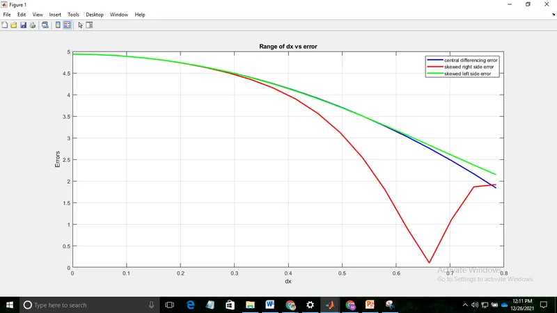
figure(1)
plot(dx, central_differencing_error, 'b', 'linewidth', 2)
hold on
plot(dx, skewed_right_side_error, 'r', 'linewidth', 2)
hold on
plot(dx, skewed_left_side_error, 'g', 'linewidth', 2)
grid on
xlabel('dx')
ylabel('Errors')
title('Range of dx vs error')
legend('central differencing error', 'skewed right side error', 'skewed left side error')

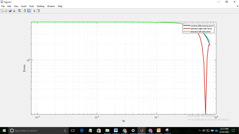
figure(2)
loglog(dx, central_differencing_error, 'b', 'linewidth', 2)
hold on
loglog(dx, skewed_right_side_error, 'r', 'linewidth', 2)
hold on
loglog(dx, skewed_left_side_error, 'g', 'linewidth', 2)
grid on
xlabel('dx')
ylabel('Errors')
legend('central differencing error', 'skewed right side error', 'skewed left side error')

Outputs:

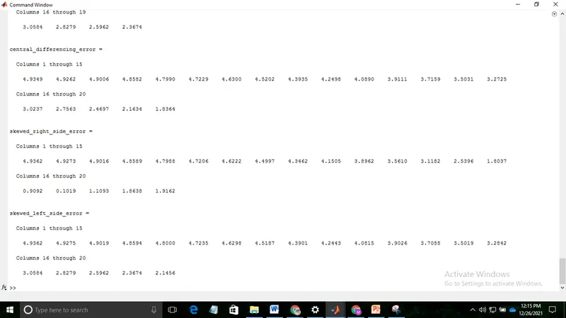
Plots:

Conclusion:

On analysing the graph, we find that central difference approximation gives more accurate solution. Hence, giving less error than skewed right and skewed left difference schemes.

Why a skewed scheme is useful:

For systems having insufficient information on both side of the point of interest, we cannot use central difference approximation in solving. So for such problems Skewed scheme are more useful.

What can a skewed scheme do that a CD scheme cannot:

Central difference schemes cannot be used at the boundary nodes due to unavailability of right or left nodes at that time. So for such problems Skewed scheme are more useful.