Week 7 - Simulation of a 1D Super-sonic nozzle flow simulation using Macormack Method
Non-Conservative governing equation.
Macormack method - aThis method is used to solve governing equation which involves 2nd order derivative without involving 2nd order derivative in solutions, thus this method simplifies the solution process. This method also give better and accurate results. There are two ways of macromack approach 'conservative' and 'non-conservative'.
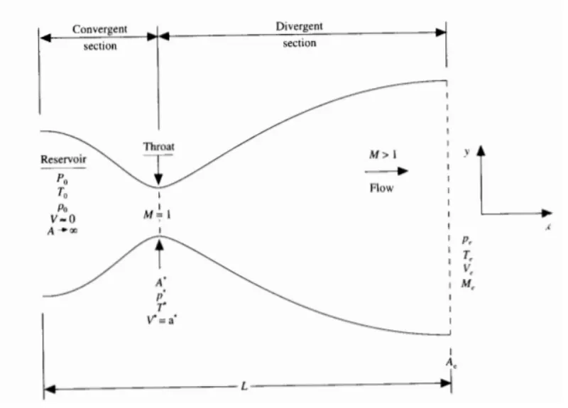
This is a 1-D supersonic convergent divergent nozzle , we will use governing equations to simulate this nozzle.
Continuity equation
`(delrho)/(delt) = -rho(delv)/(delx) - rho(del(lnA))/(delx)-v(delp)/(delx)`
Momentum equation
`(delv)/(delt) = -(delv)/(delx) - 1/r((delT)/(delx) + T/rho + (delp)/(delx))`
Energy equation
`(delT)/(delt) = -v(delT)/(delx) - (r-1)T'[(delv)/(delx) + v'(del(lnA'))/(delx)]`
Steps involved in non conservatie approach are:
- Creating mesh
- Discretize equations- during this process Macromach technique is used
- Solve
Steps involved in macromack approach:-
- Initial conditions- define initial conditions and equations for temprature ,velocity and density
- Predicted step - This step involves another 2 steps
- Discretize the equation using forward diffrencing [`(delf)/(delt)`]
- Solution update - f* = finitial + `(delf)/(delt) (trianglet)`
- corrected step - This step involves another 2 steps
- Discretize the equation using forward diffrencing [`(delf)/(delt)`]
- average of corrected and predicted step = 0.5`[(delf)/(delt)predicted + (delf)/(delt)crrected]`
In the code below we have disctretized density , velocity and energy equations by first breaking them into smaller equations
density equation = `(delrho)/(delt) = -rho(delv)/(delx) - rho(del(lnA))/(delx)-v(delp)/(delx)`
here, we will apply forward diffrencing seperattely and then add them to form complete density equation
`(delv)/(delx)` = (v(i+1) - v(i))/dx ................................1
`(delrho)/(delx)` = (rho(i+1) - rho(i))/dx`.......................2
`(del(logA))/(delx)` = (log(A(i+1) - log(A(i))/dx................3
similarly from energy equation we get
`(delT)/(delx)` = (T(i+1)-T(i))/dx....................................4
By using above equations we can simplify our density , energy and velocity equations
CODE FOR NON- conservative form of governing equations
close all
clear all
clc

%inputs
n = 31;
x = linspace(0,3,n);
dx = x(2) - x(1);
gamma = 1.4;

% calculating initial profiles
rho = 1-0.3145*x ;
T = 1-0.2314*x;
v = (0.1 + 1.09*x).*T.^0.5;
a = 1 +2.2*(x-1.5).^2; % 0 <= x <=3

%time steps
nt = 1400;

th = (n+1)/2;

%calculating dt for diffrent time steps to obtain stable solution
for i = 1:n
CFL = 0.5;

        A = sqrt(T)
        dt1(i) = CFL*dx/(A(i)+v(i))
end
dt = min(dt1);

%mach number
M= v./A;

%storing old values
rho_old = rho;
    T_old = T;
    v_old = v;
%time step loop
 for k = 1:nt

    rho_old = rho;
    T_old = T;
    v_old = v;

    %predicted method space loop
    for j = 2:n-1


        dvdx = (v(j+1)-v(j))/dx;
        drhodx = (rho(j+1)-rho(j))/dx;
        dtdx = (T(j+1)-T(j))/dx;
        dlogadx = (log(a(j+1))-log(a(j)))/dx;

        %continuity equation
        drhodt_p(j) = -rho(j)*dvdx - rho(j)*v(j)*dlogadx -v(j)*drhodx;

        %momentum equation
        dvdt_p(j) = -v(j)*dvdx - (1/gamma)*(dtdx +(T(j)/rho(j))*drhodx);

        %energy equation
        dTdt_p(j) = -v(j)*dtdx -(gamma-1)*T(j)*(dvdx + v(j)*dlogadx);
%
        %solution update
        rho(j) = rho(j)+drhodt_p(j)*dt;
        v(j) = v(j)+ dvdt_p(j)*dt;
        T(j) = T(j) + dTdt_p(j)*dt;
    end


 %corrector method space loop
    for j = 2:n-1

        dvdx = (v(j)-v(j-1))/dx;
        drhodx = (rho(j)-rho(j-1))/dx;
        dtdx = (T(j)-T(j-1))/dx;
        dlogadx = (log(a(j))-log(a(j-1)))/dx;

        %continuity equation
        drhodt_c(j) = -rho(j)*dvdx - rho(j)*v(j)*dlogadx -v(j)*drhodx;

        %momentum equation
        dvdt_c(j) = -v(j)*dvdx - (1/gamma)*(dtdx +(T(j)/rho(j))*drhodx);

        %energy equation
        dTdt_c(j) = -v(j)*dtdx -(gamma-1)*T(j)*(dvdx + v(j)*dlogadx);


    end

    %computing varegae derivative
    drhodt = 0.5*(drhodt_p + drhodt_c);
    dvdt = 0.5*(dvdt_p + dvdt_c);
    dTdt = 0.5*(dTdt_p + dTdt_c);

    %final solution update
    for i = 2:n-1
        rho(i) = rho_old(i)+ drhodt(i)*dt
        v(i) = v_old(i) + dvdt(i)*dt;
        T(i) = T_old(i) + dTdt(i)*dt;
    end

    %applying boundary condition
    %inlet
    v(1) = 2*v(2) - v(3);
    rho(1) = 1;
    T(1) = 1;

    %outlet
    v(n) = 2*v(n-1) - v(n-2);
    rho(n) = 2*rho(n-1) - rho(n-2);
    T(n) = 2*T(n-1) - T(n-2);


    %plotting steady state field variables inside nozzle

    figure(1)
    plot(x,v,'color','b')
    xlabel('length of nozzle')
    ylabel('velocity')
    legend('velocity')
    title(sprintf('time-step:%d',k))

    figure(2)
    plot(x,rho,'color','r')
    xlabel('length of nozzle')
    ylabel('density')
    legend('Density')
    title(sprintf('time-step:%d',k))

    figure(3)
    plot(x,T,'color','g')
    xlabel('length of nozzle')
    ylabel('Temprature')
    legend('Temprature')
    title(sprintf('time-step:%d',k))

    %Mass flow rate
    m = rho.*a.*v;

    %mass flow rate at throat

    rho_throat(k) = rho(th);
    v_throat(k) = v(th);
    T_throat(k) = T(th);

    %plotting mass flow rate at different time step

    figure(4)
    if k==50
        plot(x,m,'b')
        hold on
    else if k==150
        plot(x,m,'g')
        hold on
    else if k == 300
            plot(x,m,'r')
            hold on
    else if k==450
            plot(x,m,'y')
            hold on

            xlabel('nozzle length')
            ylabel('mass flow rate')
            legend('50t','150t','300t','450')
            title('Varition of mass flow at different time step')


    end
    end
    end


    end


  end


    %plotting time-wise variation of primitive variables
    figure(5)
    subplot(3,1,1)
    plot(1:k,rho_throat)
    xlabel('time variation')
    ylabel('density')
    title('Time wise variation of density')

    subplot(3,1,2)
    plot(1:k,T_throat)
    xlabel('time variation')
    ylabel('Temprature')
    title('Time wise variation of Temprature')

    subplot(3,1,3)
    plot(1:k,v_throat)
    xlabel('time variation')
    ylabel('Velocity')
    title('Time wise variation of velocity')
Explaination of code
- define all inputs such as velocity , density and temprature equations. define no of grid points
- DEfine nt(time steps)
- for dt run a loop for 1:n grid points, as we know cfl no should be less than 0.5 in order to obtain stable solution.
- start time loop which goes from 1 to nt
- store old values of density , temprature and velocity before starting space loop
- inside time loop we willplace our first space loop for predicted step, loop goes from 2:n-1 because we are doing forward differencing for interanal nodes only leaving first and last node
- Now we will start with macromach technique in which first step is predicted step
- disctretize all three governing equations and apply forward differencing
- After forward differencing , do solution update and then end predicted time step loop
- start character time step space loop , this loop also goes from 2:n-1
- character step uses backward differencing, so copy and and paste predicted step governing equations and change forward differencing with backward differencing end this loop now
- after that do averaging of predicted and corrector step solutions and a final solution update inside space loop
- define inlet and outet boundary conditions for rho , v and T
- calculate mass flow rate inside nozzle and plot mass flow rate variation at different time steps.
- plot velocity , temprature and density along length of nozzle to see their variation
- At throat value of n is n+1/2 , define field variables variables at throat
- plot field variables at throat against time variation
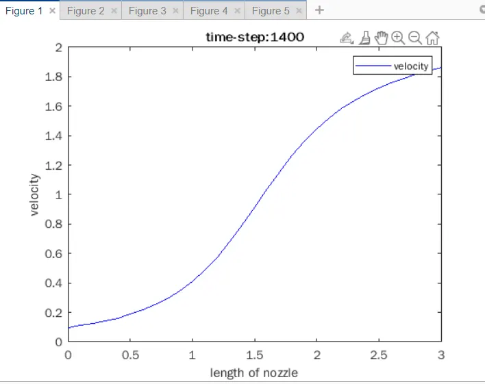
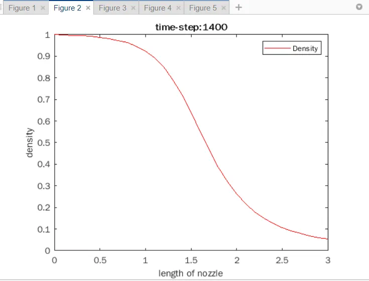
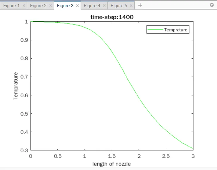
Explaination of field-variable plots-
since our nozzle is convergent -divergent type, we can observe that
- velocity increase along length of nozzle
- density and temprature drops along length of nozzle
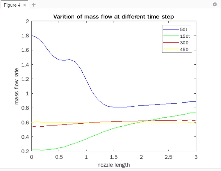
we have plot mass flow rate at different time steps to see its variation, we have observed that mass flow rate initially decreases at less time step but increases with increase in time step along length of nozzle.
we can also observe that as we approach higher time steps mass flow rate becomes horizontal which indicates that mass flow rate has reached its steady state
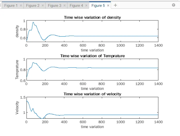
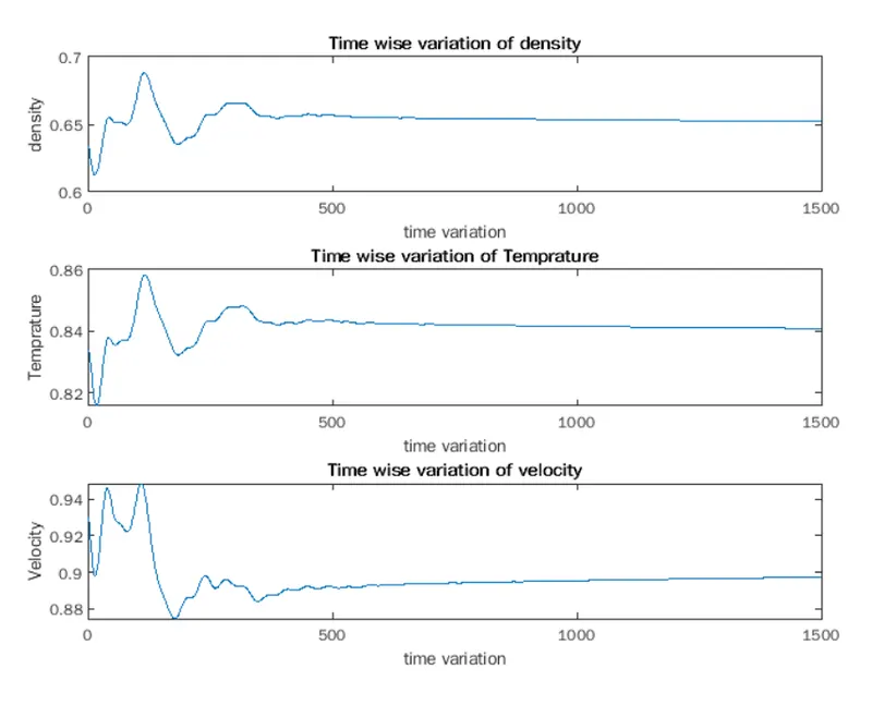
above plot shows variation of field variables at throat with time
velocity decreases at throat and density and temprature increases at throat section, this is because of shrinked area at throat section as compared to other part along length of nozzle
CONSERVATIVE FORM OF GOVERNING EQUATION:-
continuity equation = `(del(rhoA))/(delt) + (del(rhoAv))/(delx) = 0` where `(del(rhoA))/(delt) = U1, (del(rhoAv))/(delx) = F1
Momentum equation = `(del(rhoAv))/(delt) + (del[rhoAv^2 + (1/gamma)rhoA])/(delx) = (1/gamma)rho(delA)/(delx)` where,
`(del(rhoAv))/(delt) = U2 , (del[rhoAv^2 + (1/gamma)rhoA])/(delx) = F2 , (1/gamma)rho(delA)/(delx)` = J2
Energy equation = `(del[rho(e/(y-1) + gammma/2(v^2)A]))/(delt) + del[rho(e/(y-1) + gamma/2(v^2)vA+ rhoAv] = 0` where, `(del[rho(e/(y-1) + gammma/2(v^2)A]))/(delt) = U3 del[rho(e/(y-1) + gamma/2(v^2)vA+ rhoAv] = F3`
here, U = solution vector
F = flux vector
J = source vector
Generic form :-
U1 = rho*A
U2 = rho*A*v
U3 = rho(e/(gamma-1 + gamma*v^2/2)A
F1 = rhoAv
F2 = rho*A*v^2 + 1(rho*A)/gamma
F3 = rho(e/(gamma-1) + gamma*v^2/2)vA + rho*A*v
J2 = 1/gamma*rho`(delA)/(delx)`
conservative form setup
F1 = U2
F2 = U2^2/U1 + gamma-1/gamma(U3 - gamma*U2^2/2U1)
F3 = gamma(U2U3)/U1 - gamma(gamma-1)/2*U2^3/U1^2
J2 = gamma-1/gamma(U3-gamma/2*U2^2/U1) *`(del(lnA))/(delx)`
close all
clear all
clc
%inputs
L = 3;
n = 31;
x = linspace(0,3,n);
dx = x(2)-x(1);
gamma = 1.4;
A = 1+2.2*(x-1.5).^2;
nt = 1500
th = (n+1)/2;
%initial conditions
for i = 1:n
    if (x(i)>=0 && x(i) <= 0.5)
        rho(i) = 1;
        T(i) = 1;
    end
    if (x(i)>0.5) && (x(i) <= 1.5)
        rho(i) = 1 - 0.366*(x(i)- 0.5)
        T(i) = 1- 0.167*(x(i)-0.5)
    end
    if (x(i)>1.5) && (x(i)<=3)
        rho(i) = 0.634 - 0.3879*(x(i)- 1.5)
        T(i) = 0.833 - 0.3507*(x(i)-1.5)
    end
    %velocity flows along length of nozzle
    m_initial(i) = 0.59
    v(i) = m_initial(i)/(rho(i)*A(i))
end
for i = 1:n
    CFL = 0.5;
    a = sqrt(T);
    dt1(i) = CFL*dx/(a(i)+v(i));
end
dt = min(dt1)
%solution variable initialisation
U1 = rho.*A;
U2 = rho.*A.*v;
U3 = U1.*((T/(gamma-1)+(gamma/2)*v.^2));
%Predictor method
for j = 1:nt
    %storing old values
    U1_old = U1;
    U2_old = U2;
    U3_old = U3;
    %flux variable for predicted step
    F1 = U2;
    F2 = ((U2.^2)./U1)+(((gamma-1)/gamma).*(U3-((gamma*0.5*(U2.^2))./U1)));
    F3 = ((gamma.*U2.*U3)./U1) - ((0.5*gamma)*(gamma-1).*((U2.^3))./(U1.^2));
    for k = 2:n-1
        % dAdx = (A(k+1)- A(k))/dx
        % dlogAdx = (log(A(k+1))-log(A(k)))/dx
        J2(k) = (1/gamma)*rho(k)*T(k)*((A(k+1)-A(k))/dx);
        %continuity equation
        dF1dx_p = (F1(k+1)-F1(k))/dx;
        dU1dt_p(k) = -dF1dx_p;
        % momentum equation
        dF2dx_p = (F2(k+1)-F2(k))/dx;
        dU2dt_p(k) = -dF2dx_p + J2(k);

        %energy equation
        dF3dx_p = (F3(k+1)-F3(k))/dx;
        dU3dt_p(k) = -dF3dx_p;
        %step solution update
        U1(k) = (dU1dt_p(k).*dt)+U1_old(k);
        U2(k) = (dU2dt_p(k).*dt)+U2_old(k);
        U3(k) = (dU3dt_p(k).*dt)+U3_old(k);

        v(k) = U2(k)./U1(k);
        rho(k) = U1(k)./A(k);
        T(k) = (gamma-1).*((U3(k)./U1(k))-((gamma/2).*(U2(k)./U1(k)).^2));


    end

    %flux variable for corrector step
    F1 = U2;
    F2 = ((U2.^2)./U1)+(((gamma-1)/gamma).*(U3-((gamma*0.5*(U2.^2))./U1)));
    F3 = ((gamma.*U2.*U3)./U1) - ((0.5*gamma)*(gamma-1).*((U2.^3))./(U1.^2));

    for k = 2:n-1

        J2(k) = (1/gamma)*rho(k)*T(k)*((A(k)-A(k-1))/dx);
        %continuity equation
        dF1dx_c = (F1(k)-F1(k-1))/dx;
        dU1dt_c(k) = -dF1dx_c;
        %momentum equation
        dF2dx_c = (F2(k)-F2(k-1))/dx;
        dU2dt_c(k) = -dF2dx_c + J2(k);

        %energy equation
        dF3dx_c = (F3(k)-F3(k-1))/dx;
        dU3dt_c(k) = -dF3dx_c;

    end
    %computing average derivative of corrector and predictor method
    dU1dt = 0.5*(dU1dt_p + dU1dt_c);
    dU2dt = 0.5*(dU2dt_p + dU2dt_c);
    dU3dt = 0.5*(dU3dt_p + dU3dt_c);
    %final solution update
    for i = 2:n-1
        U1(i) = U1_old(i)+dU1dt(i)*dt;
        U2(i) = U2_old(i)+dU2dt(i)*dt;
        U3(i) = U3_old(i)+dU3dt(i)*dt;
    end

    %applying boundary condition
    %inlet
    U1(1) = rho(1).*A(1);
    U2(1) = 2*U2(2) - U2(3);

    v(1) = U2(1)/U1(1);
    U3(1) = U1(1)*((T(1)/(gamma-1)) + ((gamma/2)*(v(1))^2));

    %outlet
    U1(n) = (2*U1(n-1))-U1(n-2);
    U2(n) = (2*U2(n-1))-U2(n-2);
    U3(n) = (2*U3(n-1))-U3(n-2);
    %calculating primitive variables
    v = U2./U1;
    rho = U1./A;
    T = (gamma-1).*((U3./U1)-((gamma/2).*(U2./U1).^2));

    % Mass flow rate
    m = rho.*A.*v;

    %mach number
    a = sqrt(T);
    M = v./a

    %mass flow rate at throat

    rho_throat(j) = rho(th);
    v_throat(j) = v(th);
    T_throat(j) = T(th);

    %plotting mass flow rate at different time step

    figure(4)
    if j==50
        plot(x,m,'b')
        hold on
    else if j==150
        plot(x,m,'g')
        hold on
    else if j == 300
            plot(x,m,'r')
            hold on
    else if j==450
            plot(x,m,'y')
            hold on

            xlabel('nozzle length')
            ylabel('mass flow rate')
            legend('50t','150t','300t','450')
            title('Varition of mass flow at different time step')


    end
    end
    end


    end

    figure(6)
    plot(x,M,'r')
    xlabel('length of nozzle')
    ylabel('mach no')
    title('mach number')


end

    %plotting steady state field variables inside nozzle

    figure(1)
    plot(x,v,'color','b')
    xlabel('length of nozzle')
    ylabel('velocity')
    legend('velocity')
    title(sprintf('time-step:%d',k))

    figure(2)
    plot(x,rho,'color','r')
    xlabel('length of nozzle')
    ylabel('density')
    legend('Density')
    title(sprintf('time-step:%d',k))

    figure(3)
    plot(x,T,'color','g')
    xlabel('length of nozzle')
    ylabel('Temprature')
    legend('Temprature')
    title(sprintf('time-step:%d',k))


    %plotting time-wise variation of primitive variables
    figure(5)
    subplot(3,1,1)
    plot(1:j,rho_throat)
    xlabel('time variation')
    ylabel('density')
    title('Time wise variation of density')

    subplot(3,1,2)
    plot(1:j,T_throat)
    xlabel('time variation')
    ylabel('Temprature')
    title('Time wise variation of Temprature')

    subplot(3,1,3)
    plot(1:j,v_throat)
    xlabel('time variation')
    ylabel('Velocity')
    title('Time wise variation of velocity')
In conservative approach we give certain variable names to velocity , density and temprature variables to covert them into flux variables and then solve the governing equation with those choosen variables
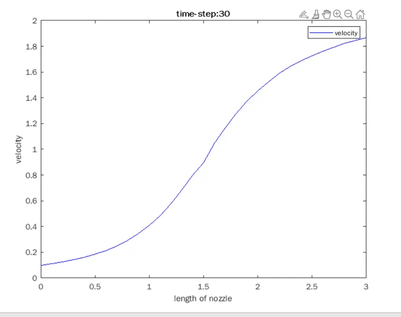
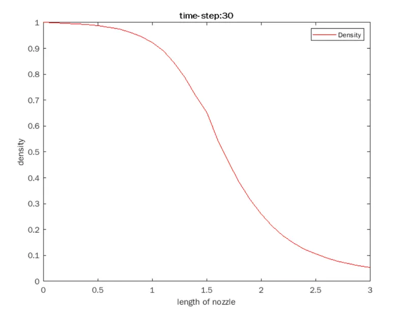
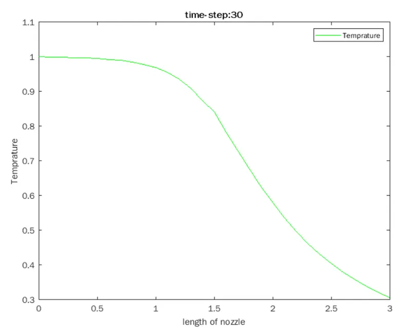
Explaination of field-variable plots-
since our nozzle is convergent -divergent type, we can observe that
- velocity increase along length of nozzle
- density and temprature drops along length of nozzle
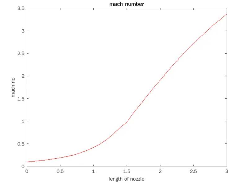
mach no increases along length of nozzle which indictes solution reaching stability
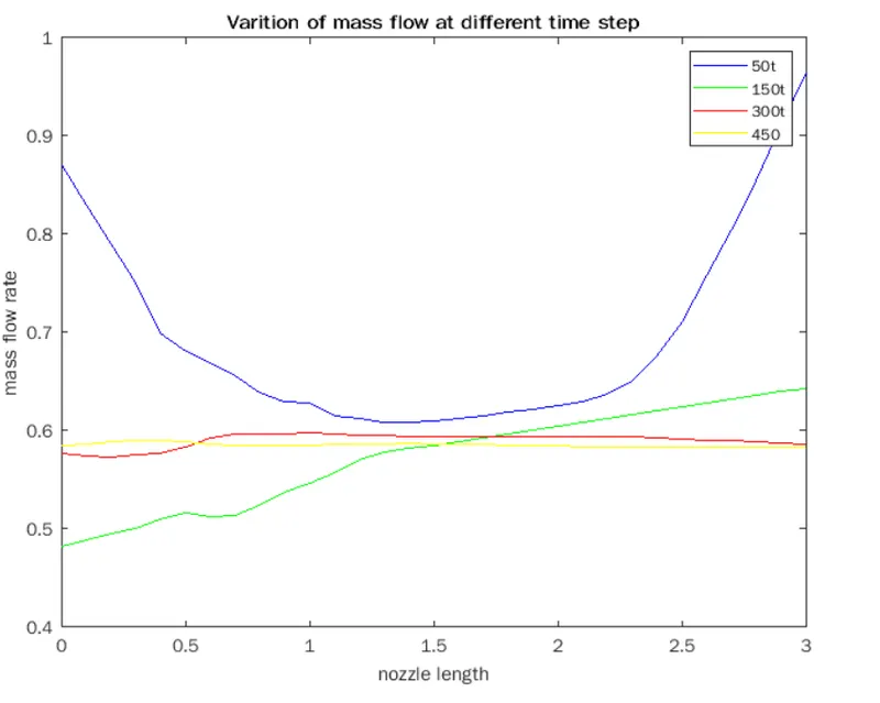
we have plot mass flow rate at different time steps to see its variation, we have observed that mass flow rate initially decreases at less time step but increases with increase in time step along length of nozzle.
we can also observe that as we approach higher time steps mass flow rate becomes horizontal which indicates that mass flow rate has reached its steady state
Conclusion-
- if we compare conservative and non- conservative approach , we can observe that non-conservative form of approach is more close to exact solution
- so we can conclude that non_conservative approach is much easier to code and understand than conservative approach.