Week 5.1 - Mid term project - Solving the steady and unsteady 2D heat conduction problem

CODE FOR STEADY STATE HEAT CONDUCTION EQUATION USING

1. JACOBI ITERATION METHOD
2. GAUSS SEIDEL METHOD
3. SOR ITERATION METHOD

Steady state heat conduction equation:

`(del^2T)/(delx^2) + (del^2T)/(dely^2) = 0 or triangleT = 0`

after solving and discretising above equation we get,

T = 1/k((T_L + T_R)/`trianglex^2`) + 1/k((T_T+ T_B)/`triangley^2`),

where k = `(2(trianglex^2 + triangley^2))/(trianglex^2y^2`

Tempratures at top left rright anf left of matrix

Top Boundary = 600 K

Bottom Boundary = 900 K

Left Boundary = 400 K

Right Boundary = 800 K

BELOW IS THE CODE FOR STEADY STATE HEAT CONDUCTION

close all
clear all
clc

% jacobi iteration method
 %inputs
 L = 1;
 nx=20;
 ny = 20;
 x = linspace(0,L,nx);
 y = linspace(0,L,ny);

 dx = x(2) - x(1);
 dy = y(2) - y(1);

 error = 9e9
 %initial tempratures along matrix
 T = ones(nx,ny);
 %input tempratures
 T_L = 400;
 T_T = 600;
 T_B = 900;
 T_R = 800;

 %tempratures along boundary
 T(2:ny-1,1) = T_L;
 T(2:ny-1,nx) = T_R;
 T(1,2:nx-1) = T_T;
 T(nx,2:ny-1) = T_B;

 %tempratures along corners
 T(1,1) = (T_T + T_L)/2;
 T(nx,ny) = (T_R + T_B)/2;
 T(1,ny) = (T_T+T_R)/2;
 T(nx,1) = (T_L + T_B)/2;

 k1 = (dy^2)/(2*(dx^2 + dy^2));

 k2 = (dx^2)/(2*(dx^2 + dy^2));

 %creating mesh 
 [X,Y] = meshgrid(x,y);

 Told = T;
 tol = 1e-4;

 for iterative_solver = 1
     tic
     if iterative_solver == 1
         jacobi_iter = 1;
         while( error > tol)
             for i = 2:nx-1
                 for j = 2:ny-1
                     T(i,j) = k1*(Told(i-1,j) + Told(i+1,j)) + k2*(Told(i,j-1) + Told(i,j+1)); 
                 end
             end
             error = max(max(abs(Told-T)));
             Told = T;
             jacobi_iter = jacobi_iter + 1;
         end
     end
     time_required = toc;
     %plotting
     figure(1)
     [a,b] = contourf(X,Y,T)
     colorbar
     clabel(a,b)
     xlabel = ('x axis')
     ylabel = ('y axis')

     title_text1 = sprintf('steady state - jacobi method')
     title_text2 = sprintf('no of iteration = %d',jacobi_iter)
     title({title_text1,title_text2})
 end

 % gaus seidel method
 %inputs
 L = 1;
 nx=20;
 ny = 20;
 x = linspace(0,L,nx);
 y = linspace(0,L,ny);

 dx = x(2) - x(1);
 dy = y(2) - y(1);

 error = 9e9
 %initial tempratures along matrix
 T = ones(nx,ny);
 %input tempratures
 T_L = 400;
 T_T = 600;
 T_B = 900;
 T_R = 800;

 %tempratures along boundary
 T(2:ny-1,1) = T_L;
 T(2:ny-1,nx) = T_R;
 T(1,2:nx-1) = T_T;
 T(nx,2:ny-1) = T_B;

 %tempratures along corners
 T(1,1) = (T_T + T_L)/2;
 T(nx,ny) = (T_R + T_B)/2;
 T(1,ny) = (T_T+T_R)/2;
 T(nx,1) = (T_L + T_B)/2;

 k1 = (dy^2)/(2*(dx^2 + dy^2));

 k2 = (dx^2)/(2*(dx^2 + dy^2));

 %creating mesh 
 [X,Y] = meshgrid(x,y);

 Told = T;
 tol = 1e-4;

 for iterative_solver = 1
     tic
     if iterative_solver == 1
         gaus_iter = 1;
         while( error > tol)
             for i = 2:nx-1
                 for j = 2:ny-1
                     T(i,j) = k1*(T(i-1,j) + T(i+1,j)) + k2*(T(i,j-1) + T(i,j+1)); 
                 end
             end
             error = max(max(abs(Told-T)));
             Told = T;
             gaus_iter = gaus_iter + 1;
         end
     end
     time_required = toc;
     %plotting
     figure(2)
     [a,b] = contourf(X,Y,T)
     colorbar
     clabel(a,b)
     xlabel = ('x axis')
     ylabel = ('y axis')

     title_text1 = sprintf('steady state - gaus method')
     title_text2 = sprintf('no of iteration = %d',gaus_iter)
     title({title_text1,title_text2})
 end

 %SOR iteration method 
  %inputs
 L = 1;
 nx=20;
 ny = 20;
 x = linspace(0,L,nx);
 y = linspace(0,L,ny);

 dx = x(2) - x(1);
 dy = y(2) - y(1);

 error = 9e9
 %initial tempratures along matrix
 T = ones(nx,ny);
 %input tempratures
 T_L = 400;
 T_T = 600;
 T_B = 900;
 T_R = 800;

 %calculation omega
 omega = 1.1

 %tempratures along boundary
 T(2:ny-1,1) = T_L;
 T(2:ny-1,nx) = T_R;
 T(1,2:nx-1) = T_T;
 T(nx,2:ny-1) = T_B;

 %tempratures along corners
 T(1,1) = (T_T + T_L)/2;
 T(nx,ny) = (T_R + T_B)/2;
 T(1,ny) = (T_T+T_R)/2;
 T(nx,1) = (T_L + T_B)/2;

 k1 = (dy^2)/(2*(dx^2 + dy^2));

 k2 = (dx^2)/(2*(dx^2 + dy^2));

 %creating mesh 
 [X,Y] = meshgrid(x,y);

 Told = T;
 tol = 1e-4;

 for iterative_solver = 1
     tic
     if iterative_solver == 1
         SOR_iter = 1;
         while( error > tol)
             for i = 2:nx-1
                 for j = 2:ny-1
                     T(i,j) = (1-omega)*Told(i,j) + omega*( k1*(T(i-1,j) + T(i+1,j)) + k2*(T(i,j-1) + T(i,j+1))); 
                 end
             end
             error = max(max(abs(Told-T)));
             Told = T;
             SOR_iter = SOR_iter + 1;
         end
     end
     time_required = toc;
     %plotting
     figure(3)
  
     [a,b] = contourf(X,Y,T)
     colorbar
     clabel(a,b)
     xlabel = ('x axis')
     ylabel = ('y axis')

     title_text1 = sprintf('steady state - SOR method')
     title_text2 = sprintf('no of iteration = %d',SOR_iter)
     title({title_text1,title_text2})
 end

Explaination of code:-

• Give inputs for L , L is a square area of 1m sides along which heat conduction would take place
• nx and ny are no of nodes in which square surface is divided along x and y axis
• use linspace command divide x and y axis into equal nodes
• use meshgrid command to create a mesh of nx and ny
• define Tempratures on top , bottom ,right and left of our surface. use tempratures to calculate tempratures at corners of square matrix and along x and y boundary length of our matrix
• T = ones(nx,ny) is used to define initial temprature condition along nx and ny or it is the temprature at mid of matrix
• define or error and tolerance, error should be greater than tolerance

There are total three methods used in code , we will explain each method one by one

JACOBI ITERATION

• After giving all inputs , assign new value to T which is Told
• In jacobi method we use initial values or Told value to find new values of T
• on the RHS Told values would we used
• start define our loops , there are of total 5 loops which we will use
• start with defining iteration number, there are 3 iteration method we are using, hence for each iteration we will assign a number as 1, 2, 3
• since jacobi is our first iteration hence its iteration number is 1
• after that is our if loop, this loop is used to confirm that we are using iteration of which number
• after that is our while loop, this loops says our iteration will run until error>tolerance
• after that comes our space loop, here we will define loop conditions along x and y
• x and y loop are running from 2:nx-1 and 2:ny-1, which means we want to calculate tempratures from 2nd point on nx and ny to 2nd last point. we have done so because we already know tempratures on boundaries
• inside this loop we willl use our jacobi formula, as you can see on RHS Told values are used. close space loop.
• After space loop calculate error, we are using max two times because this is a 2D problem
• Restore Told values
• jacobi_iter = jacobi_iter+1 is used to calculate no of iterations used in calculation of Tnew
• close if loop and while loop
• plot the values of T in our mesh X,Y
• use conntourf command to display variation T along x and y axis in [X,Y]mesh
• [a,b] on LHS is used to assign and show temprature values in plot

GAUS SEIDEL ITERATION

• After giving all inputs , assign new value to T which is Told
• In jacobi method we use initial values or Told value to find new values of T
• on the RHS T values would we used
• start define our loops , there are of total 5 loops which we will use
• start with defining iteration number, there are 3 iteration method we are using, hence for each iteration we will assign a number as 1, 2, 3
• since jacobi is our first iteration hence its iteration number is 1
• after that is our if loop, this loop is used to confirm that we are using iteration of which number
• after that is our while loop, this loops says our iteration will run until error>tolerance
• after that comes our space loop, here we will define loop conditions along x and y
• x and y loop are running from 2:nx-1 and 2:ny-1, which means we want to calculate tempratures from 2nd point on nx and ny to 2nd last point. we have done so because we already know tempratures on boundaries
• inside this loop we willl use our gaus formula, as you can see on RHS T values are used. close space loop.
• After space loop calculate error, we are using max two times because this is a 2D problem
• Restore Told values
• gaus_iter = gaus_iter+1 is used to calculate no of iterations used in calculation of Tnew
• close if loop and while loop
• plot the values of T in our mesh X,Y
• use conntourf command to display variation T along x and y axis in [X,Y]mesh
• [a,b] on LHS is used to assign and show temprature values in plot

SOR ITERATION METHOD

• In sor method a term omega is introduced
• omega is known is relaxation factor, this iteration method is more than gaus and jacobi method
• if omega<1 it is under relaxation
• if omega >1 it is over relaxation
• use value of omega which is close to 1, as it will give more accurate results and in less number of iterations
• eveything would be same , just use sor fromula inside space loop

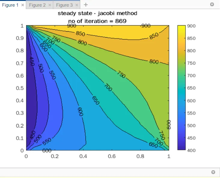
JACOBI ITERATION METHOD

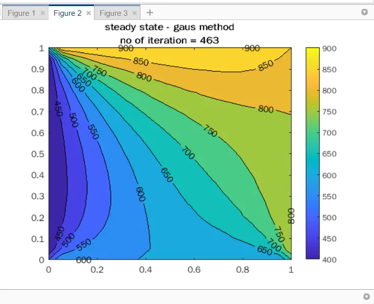
GAUSS ITERATION METHOD

SOR ITERATION METHOD

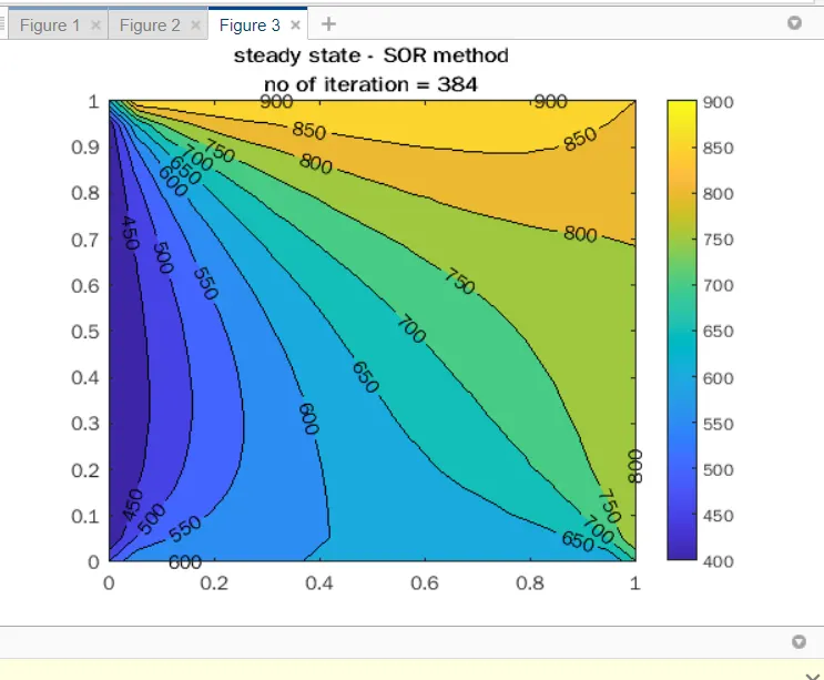
Iteration numbers follow a sequence which

jacobi iteration>gaus iteration>sor iteration

sor technique much less iteration than other two and is more advanced.

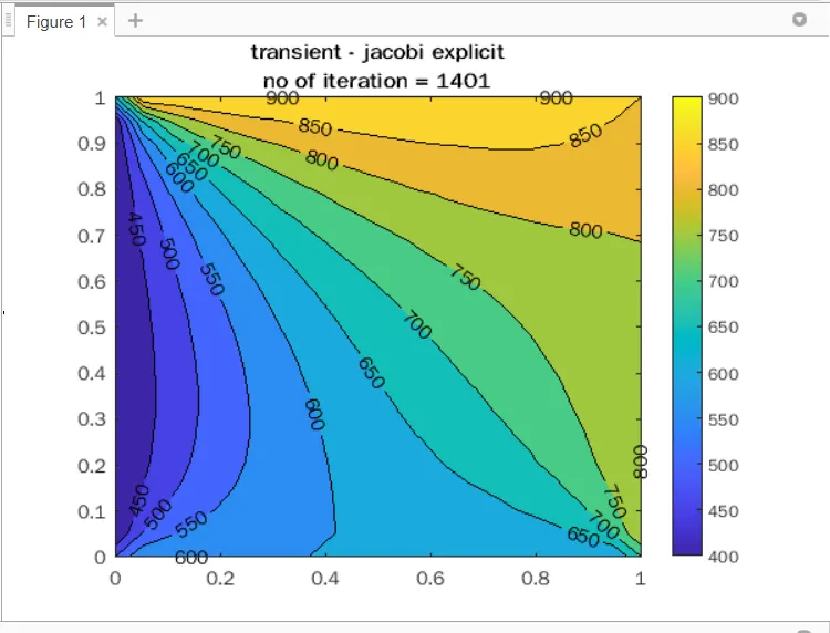
CODE FOR TRANSIENT HEAT CONDUCTION USING EXPLICIT SCHEMES

close all
clear all
clc

% jacobi iteration method for transient condition (explicit scheme)
 %inputs
 L = 1;
 nx=20;
 ny = 20;
 x = linspace(0,L,nx);
 y = linspace(0,L,ny);

 dx = x(2) - x(1);
 dy = y(2) - y(1);

 error = 9e9;
 alpha = 1.4;
 % no of time steps
 dt = 40;
 nt = 1400;
 %initial tempratures along matrix
 T = ones(nx,ny);
 %input tempratures
 T_L = 400;
 T_T = 600;
 T_B = 900;
 T_R = 800;

 %tempratures along boundary
 T(2:ny-1,1) = T_L;
 T(2:ny-1,nx) = T_R;
 T(1,2:nx-1) = T_T;
 T(nx,2:ny-1) = T_B;

 %tempratures along corners
 T(1,1) = (T_T + T_L)/2;
 T(nx,ny) = (T_R + T_B)/2;
 T(1,ny) = (T_T+T_R)/2;
 T(nx,1) = (T_L + T_B)/2;

 k1 = (alpha*dt/(dx^2));
 k2 = (alpha*dt/(dy^2));

 %creating mesh 
 [X,Y] = meshgrid(x,y);

 Told = T;
 tol = 1e-4;
Tprev_dt = Told;

 
     
     
     
         jacobi_iter = 1;
         for nt = 1:1400
             for i = 2:nx-1
                 for j = 2:ny-1
                     term1 = (1+(2*k1)+(2*k2))^-1;
                     term2 = k1*term1;
                     term3 = k2*term1;
                     H = (Told(i-1,j) +Told(i+1,j));
                     V = (Told(i,j-1)+Told(i,j+1));
                     T(i,j) = (Told(i,j)*term1)+(H*term2)+ (V*term3);
                     
                     

                      
                 end
             end
             
             Told = T;
             
           
             jacobi_iter = jacobi_iter + 1;
         
     
     time_required = toc;
     %plotting
     figure(1)
     [a,b] = contourf(X,Y,T)
     colorbar
     clabel(a,b)
     xlabel = ('x axis')
     ylabel = ('y axis')

     title_text1 = sprintf('transient - jacobi explicit')
     title_text2 = sprintf('no of iteration = %d',jacobi_iter)
     title({title_text1,title_text2})
         end
 

CODE FOR TRANSIENT STATE HEAT CONDUCTION USING IMPLICIT SCHEME:

Formula for transient state 2 D heat conductionn equation is

`(delT)/(delt) + alpha( (del^2T)/(delx^2) + (del^2T)/(dely^2)) = 0`

method used

1. jacobi iteration method
2. gauss iteration method
3. sor iteration method

Below is the code for implicit scheme

close all 
clear all
clc

%JACOBI ITERATION
%inputs
 L = 1;
 nx=20;
 ny = 20;
 x = linspace(0,L,nx);
 y = linspace(0,L,ny);

 dx = x(2) - x(1);
 dy = y(2) - y(1);

 error = 9e9;
 alpha = 1.4;
 % no of time steps
 dt = 40;
 nt = 1400;
 %initial tempratures along matrix
 T = ones(nx,ny);
 %input tempratures
 T_L = 400;
 T_T = 600;
 T_B = 900;
 T_R = 800;

 %tempratures along boundary
 T(2:ny-1,1) = T_L;
 T(2:ny-1,nx) = T_R;
 T(1,2:nx-1) = T_T;
 T(nx,2:ny-1) = T_B;

 %tempratures along corners
 T(1,1) = (T_T + T_L)/2;
 T(nx,ny) = (T_R + T_B)/2;
 T(1,ny) = (T_T+T_R)/2;
 T(nx,1) = (T_L + T_B)/2;

 k1 = (alpha*dt/(dx^2));
 k2 = (alpha*dt/(dy^2));

 %creating mesh 
 [X,Y] = meshgrid(x,y);

 Told = T;
 tol = 1e-4;
Tprev_dt = T;
for iterative_solver =1;
    tic
    if iterative_solver == 1;


jacobi_iter = 1;
for nt = 1:1400
    error = 9e9;
 
     
     
         
         while( error > tol)
             for i = 2:nx-1
                 for j = 2:ny-1
                     term1 = (1+(2*k1)+(2*k2))^-1;
                     term2 = k1*term1;
                     term3 = k2*term1;
                     H = (Told(i-1,j) +Told(i+1,j));
                     V = (Told(i,j-1)+Told(i,j+1));
                     T(i,j) = (Tprev_dt(i,j)*term1)+(H*term2)+ (V*term3);
                 
                 end
             end
             error = max(max(abs(Told-T)));
             Told = T;
             
           
             jacobi_iter = jacobi_iter + 1;
         end
         tprev_dt = T;
         time_required = toc;
     %plotting
     figure(1)
     [a,b] = contourf(X,Y,T)
     colorbar
     clabel(a,b)
     xlabel = ('x axis')
     ylabel = ('y axis')

     title_text1 = sprintf('transient - jacobi imlicit')
     title_text2 = sprintf('no of iteration = %d',jacobi_iter)
     title({title_text1,title_text2})

end
    end
end
     
%GAUS SEIDEL ITERATION
%inputs
 L = 1;
 nx=20;
 ny = 20;
 x = linspace(0,L,nx);
 y = linspace(0,L,ny);

 dx = x(2) - x(1);
 dy = y(2) - y(1);

 error = 9e9;
 alpha = 1.4;
 % no of time steps
 dt = 40;
 nt = 1400;
 %initial tempratures along matrix
 T = ones(nx,ny);
 %input tempratures
 T_L = 400;
 T_T = 600;
 T_B = 900;
 T_R = 800;

 %tempratures along boundary
 T(2:ny-1,1) = T_L;
 T(2:ny-1,nx) = T_R;
 T(1,2:nx-1) = T_T;
 T(nx,2:ny-1) = T_B;

 %tempratures along corners
 T(1,1) = (T_T + T_L)/2;
 T(nx,ny) = (T_R + T_B)/2;
 T(1,ny) = (T_T+T_R)/2;
 T(nx,1) = (T_L + T_B)/2;

 k1 = (alpha*dt/(dx^2));
 k2 = (alpha*dt/(dy^2));

 %creating mesh 
 [X,Y] = meshgrid(x,y);

 Told = T;
 tol = 1e-4;
Tprev_dt = T;
for iterative_solver =1;
    tic
    if iterative_solver == 1;


gaus_iter = 1;
for nt = 1:1400
    error = 9e9;
 
     
     
         
         while( error > tol)
             for i = 2:nx-1
                 for j = 2:ny-1
                     term1 = (1+(2*k1)+(2*k2))^-1;
                     term2 = k1*term1;
                     term3 = k2*term1;
                     H = (T(i-1,j) +T(i+1,j));
                     V = (T(i,j-1)+T(i,j+1));
                     T(i,j) = (Tprev_dt(i,j)*term1)+(H*term2)+ (V*term3);
                 
                 end
             end
             error = max(max(abs(Told-T)));
             Told = T;
             
           
             gaus_iter = gaus_iter + 1;
         end
         tprev_dt = T;
         time_required = toc;
     %plotting
     figure(2)
     [a,b] = contourf(X,Y,T)
     colorbar
     clabel(a,b)
     xlabel = ('x axis')
     ylabel = ('y axis')

     title_text1 = sprintf('transient - Gauss imlicit')
     title_text2 = sprintf('no of iteration = %d',gaus_iter)
     title({title_text1,title_text2})

end
    end
end

%SOR IMPLICIT ITERATION
%inputs
 L = 1;
 nx=20;
 ny = 20;
 x = linspace(0,L,nx);
 y = linspace(0,L,ny);

 dx = x(2) - x(1);
 dy = y(2) - y(1);

 error = 9e9;
 alpha = 1.4;
 omega = 1.1;
 % no of time steps
 dt = 40;
 nt = 1400;
 %initial tempratures along matrix
 T = ones(nx,ny);
 %input tempratures
 T_L = 400;
 T_T = 600;
 T_B = 900;
 T_R = 800;

 %tempratures along boundary
 T(2:ny-1,1) = T_L;
 T(2:ny-1,nx) = T_R;
 T(1,2:nx-1) = T_T;
 T(nx,2:ny-1) = T_B;

 %tempratures along corners
 T(1,1) = (T_T + T_L)/2;
 T(nx,ny) = (T_R + T_B)/2;
 T(1,ny) = (T_T+T_R)/2;
 T(nx,1) = (T_L + T_B)/2;

 k1 = (alpha*dt/(dx^2));
 k2 = (alpha*dt/(dy^2));

 %creating mesh 
 [X,Y] = meshgrid(x,y);

 Told = T;
 tol = 1e-4;
Tprev_dt = T;

for iterative_solver =3;
    tic
    if iterative_solver == 3;


sor_iter = 1;
for nt = 1:1400
    error = 9e9;
 
     
     
         
         while( error > tol)
             for i = 2:nx-1
                 for j = 2:ny-1
                     term1 = (1+(2*k1)+(2*k2))^-1;
                     term2 = k1*term1;
                     term3 = k2*term1;
                     H = (T(i-1,j) +T(i+1,j));
                     V = (T(i,j-1)+T(i,j+1));
                     T(i,j) = (1-omega)*Told(i,j) + omega*((Tprev_dt(i,j)*term1)+ (H*term2)+ (V*term3));
                 
                 end
             end
             error = max(max(abs(Told-T)));
             Told = T;
             
           
             sor_iter = sor_iter + 1;
         end
         tprev_dt = T;
         time_required = toc;
     %plotting
     figure(3)
     [a,b] = contourf(X,Y,T)
     colorbar
     clabel(a,b)
     xlabel = ('x axis')
     ylabel = ('y axis')

     title_text1 = sprintf('transient - jacobi imlicit')
     title_text2 = sprintf('no of iteration = %d',sor_iter)
     title({title_text1,title_text2})

end
    end
end

Explaination od code:-

• In implicit scheme we dont know value of T at RHS in equation.
• use of time step is introduced in implicit schemes to fin new values of T.
• we use time loop, convergence loop , space loop , for loops and iterative condition loops
• first start with iterative loop, inside this loop second loop would be if iterative loop to define which iterative solver technique we are using
• after that is our time loop, this defines the no time time steps our solution will converge
• after that is our convergence loop , this loop defines condition fr how long our convergence shoild take place. Here, convergence should take place until error is greater than tolerance
• after that is our for loop for nx and ny . Inside for loop we will place our formula to calculate values of T, both for loops for nx and ny would close after writing formula inside them

Lets discuss how formula for jacobi , gaus and sor varies

Jacobi

• In jacobi we will use Told values on RHS

gauss

• In gauss T values are on RHS, which means after each iteration pervious value of T is used which we got after that iteration took place

SOR

• In sor a term omega is introduced. omega is relaxation factor
• if omega > 1, it is over relaxation
• if omega <1 it is under relaxation
• use value of omega close to 1 to get better results

plotting:

• plot the values of T in our mesh X,Y
• use conntourf command to display variation T along x and y axis in [X,Y]mesh
• [a,b] on LHS is used to assign and show temprature values in plot
• use labels to define x and y axis
• give iterative solver=%d to define number of iterations on plot

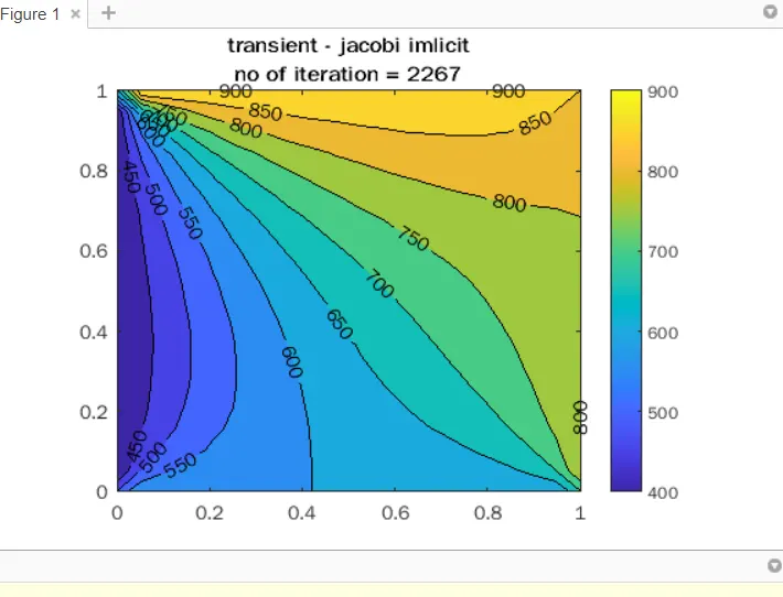
JACOBI ITERATION IMPLICIT

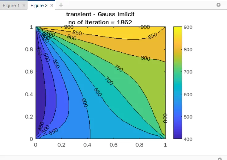
GAUSS ITERATION IMPLICIT

SOR ITERATION IMPLICIT

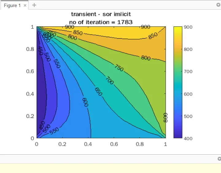
Iteration numbers follow a sequence which

jacobi iteration>gaus iteration>sor iteration

sor technique much less iteration than other two and is more advanced. SOR technique uses much less iteration to converge a equation than jacobi and gauss