Week 4.1 - Genetic Algorithm

WHAT IS OPTIMISATION:

Optimisation is technique to find optimum solution or near optimum solution to given problem. eg: you want a minimum possible value of drag coefficient for a particular shape, the value of parameters which define drag coefficient can be choosen with help of optimisation.

WHAT IS GENETIC ALGORITHM:

Genetic algorithm is based on darwin's theory of evolution, which explains the fittest would survive. GA is one of the processes to achieve optimisation.

GA constitues of 5 processes-

• Initial Population - A set of individual genes is taken into consideration. each set of genes has its own characteristics
• Fitness function - this function is used to evaluate how much a given solution is near to an optimum solution. Each solution is awarded a fitness score based on how much they are close optimum solution.
• Selection - This process picks up the fittests individuals and let them pass their genes to next generation. Individuals are picked on basis of their fitness score, best score ones are picked.
• Crossover- It is most important point in GA, for each pair of genes mutated a cross over point is choosen at random within genes.
• MUtation- This is required so that genes produced are different from each other and does not poses similar properties. It is achieved by increasing population size to get maximum diversity

GA syntax-

we will discuss three syntax we used in our code

• [x] = ga(fun,nvar), finds a local unconstrained minimum x to function fun. nvars is no design variables in fun

• [x] = ga(fun,nvar,A,b,lb,ub), finds a constrained minimum at x to function fun subjected to linear inequalities A*x<b.ga evalutes matrix A*x as if transposed. nvars is a design variables in fun.

• [x] = ga(fun,nvar,A,b,Aeq,beq,) , finds a constrained minimum at x to function fun subjected to linear equalities Aeq = beq, put A & b as [],[] if no linear inequalities exists.

• [x] = ga(fun,nvar,A,b,Aeq,beq,lb,ub), defies a set of lower and upper bound on design variable x so solution is range between lb and ub. put Aeq, beq, A, b as [],[],[],[] if no linear equalities nad inequalities exists.

• [x] = ga(fun,nvar,A,b,Aeq,beq,lb,ub,nonIcon,options) , used to give increased population size, use noIcon as [] if no linear constraints exist.

• [x,fval] = ga(____), gives values of fval at input x

LETS,S MOVE TO CODING PART.

Stlagmite function code-

 
 function   [S] = stalagmite_fun(input_vector)
x = input_vector(1);
y = input_vector(2);
 
 f1x = (sin((5.1*3.14).*x+ 0.5)).^6;
 f1y = (sin((5.1*3.14).*y+ 0.5)).^6;
 
 f2x = exp((-4*log(2)) *((x-0.667).^2)/0.64);
 f2y = exp((-4*log(2)) *((y-0.667).^2)/0.64);
 
 S = -(f1x*f1y*f2x*f2y);
 end

Here, x & y are variables which are inputs to the function.

since ga minimises a function, we are using (-) sign in S= -(f1x*f1y*f2x*f2y), so that ga automatically gives maximum value to our function

Program code-

close all
clear all
clc

x = linspace(0,0.6,120);
y = linspace(0,0.6,120);

[xx yy] = meshgrid(x,y);

num_spaces = 55

for i = 1:length(x)
    for j = 1:length(y)
        input_vector(1) = xx(i,j);
        input_vector(2) = yy(i,j);
       f(i,j) = stalagmite_fun(input_vector);
       
    end
end

% study 1 unbounded solution
tic
for i = 1:num_spaces
    [inputs,fopt(i)] = ga(@stalagmite_fun,2);
    xopt(i) = inputs(1);
    yopt(i) = inputs(2);
end
studytime_1 = toc

subplot(2,1,1)
surface(x,y,-f)
shading interp
xlabel('x value')
ylabel('y value')
title('genetic algorithm')
hold on
plot3(xopt,yopt,-fopt,'marker','o')
subplot(2,1,2)
plot(fopt)
xlabel('iteration')
ylabel('maximum values')

% iteration for bounded values
tic
for i = 1:num_spaces
    [inputs,fopt(i)] = ga(@stalagmite_fun,2,[],[],[],[],[0;0],[0.6;0.6]);
    xopt(i) = inputs(1);
    yopt(i) = inputs(2);
end 
studytime_2 = toc
figure(2)
subplot(2,1,1)
surface(x,y,-f)
shading interp
title('genetic algorithm')
xlabel('x value')
ylabel('y value')
hold on
plot3(xopt,yopt,-fopt,'marker','o')
subplot(2,1,2)
plot(fopt)
xlabel('iteration')
ylabel('maximum value')
%bounded with increased population 
tic
options = optimoptions('ga')
options = optimoptions(options,'populationsize',300)

for i = 1:num_spaces
    [inputs,fopt(i)] = ga(@stalagmite_fun,2,[],[],[],[],[0;0],[0.6;0.6],[],[],options);
    xopt(i)=inputs(1);
    yopt(i)=inputs(2);
end
studytime_4=toc
figure(3)
subplot(2,1,1)
surface(x,y,-f)
title('genetic algorithm')
xlabel('x value')
ylabel('y value')
shading interp
hold on
plot3(xopt,yopt,-fopt,'marker','o')
subplot(2,1,2)
plot(fopt)
xlabel('iteration')
ylabel('maximum value')

Explaination of code-

[xx yy] = meshgrid(x,y)

we need to create 2D array from x & y for that we will use meshgrid command.

num_spaces = 55

for i = 1:length(x)
for j = 1:length(y)
input_vector(1) = xx(i,j);
input_vector(2) = yy(i,j);
f(i,j) = stalagmite_fun(input_vector);

end
end

num spaces - we need the iteration to run 55 times

we have used for loop command and save the 2D array in input_vector so it can be used to call stalagmite function.

for 1st iteration,unbounded iteration

% study 1 unbounded solution
tic
for i = 1:num_spaces
[inputs,fopt(i)] = ga(@stalagmite_fun,2);
xopt(i) = inputs(1);
yopt(i) = inputs(2);
end
studytime_1 = toc

subplot(2,1,1)
surface(x,y,-f)
shading interp
hold on
plot3(xopt,yopt,-fopt,'marker','o')
subplot(2,1,2)
plot(fopt)
xlabel('iteration')
ylabel('maximum values')

num_spaces = no of iterations

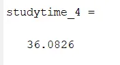
tic & toc command is used to calculate the time taken taken for iteration.

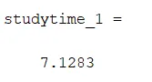
values of inputs are used to get values for fopt, these values of fopt are saved in xopt & yopt

To create a 3d plot we will use surface command and our 3dimensional values are x,y&-f

subplot command is used when we need to give 2 plots in a single frame, subplot(2,1,1) displays 2 rows 1 column & 1st figure

shading interp is used to get a clear & smoother plot free of shading lines.

plot3 command is also used to create a plot with 3 input values. by this plot we will show all the optimum values ga function gives.

plot(fopt) is our second plot thats why subplot(2,1,2) is used before giving this command. we will plot all values of fopt we got.

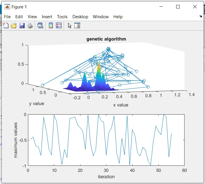
This is the plot we got in our 1st iteration, as you cansee this plot isshowing many optimum values on which we cannot rely on , so we will go with firther iteration.

2nd iteration , bounded iteration

% iteration for bounded values
tic
for i = 1:num_spaces
    [inputs,fopt(i)] = ga(@stalagmite_fun,2,[],[],[],[],[0;0],[0.6;0.6]);
    xopt(i) = inputs(1);
    yopt(i) = inputs(2);
end 
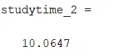
studytime_2 = toc
figure(2)
subplot(2,1,1)
surface(x,y,-f)
shading interp
title('genetic algorithm')
xlabel('x value')
ylabel('y value')
hold on
plot3(xopt,yopt,-fopt,'marker','o')
subplot(2,1,2)
plot(fopt)
xlabel('iteration')
ylabel('maximum value')

num_spaces = no of iteration

here, [inputs,fopt(i)] = ga(@stalagmite_fun,2,[],[],[],[0;0],[0.6;0.6]);

values of inputs are used to get values for fopt, these values of fopt are saved in xopt & yopt

To create a 3d plot we will use surface command and our 3dimensional values are x,y&-f

subplot command is used when we need to give 2 plots in a single frame, subplot(2,1,1) displays 2 rows 1 column & 1st figure

shading interp is used to get a clear & smoother plot free of shading lines.

plot3 command is also used to create a plot with 3 input values. by this plot we will show all the optimum values ga function gives.

plot(fopt) is our second plot thats why subplot(2,1,2) is used before giving this command. we will plot all values of fopt we got.

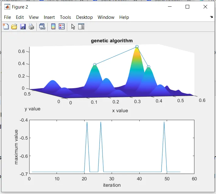
We are getting 3 values for fopt which means 2 optiimum values, so we will gowith firther iteration

3rd iteration with increased population size

%bounded with increased population 
tic
options = optimoptions('ga')
options = optimoptions(options,'populationsize',300)

for i = 1:num_spaces
    [inputs,fopt(i)] = ga(@stalagmite_fun,2,[],[],[],[],[0;0],[0.6;0.6],[],[],options);
    xopt(i)=inputs(1);
    yopt(i)=inputs(2);
end
studytime_4=toc
figure(3)
subplot(2,1,1)
surface(x,y,-f)
title('genetic algorithm')
xlabel('x value')
ylabel('y value')
shading interp
hold on
plot3(xopt,yopt,-fopt,'marker','o')
subplot(2,1,2)
plot(fopt)
xlabel('iteration')
ylabel('maximum value')

In this command we have used optimoptions command to increase our population size to 250

values of inputs are used to get values for fopt, these values of fopt are saved in xopt & yopt

To create a 3d plot we will use surface command and our 3dimensional values are x,y&-f

subplot command is used when we need to give 2 plots in a single frame, subplot(2,1,1) displays 2 rows 1 column & 1st figure

shading interp is used to get a clear & smoother plot free of shading lines.

plot3 command is also used to create a plot with 3 input values. by this plot we will show all the optimum values ga function gives.

plot(fopt) is our second plot thats why subplot(2,1,2) is used before giving this command. we will plot all values of fopt we got.

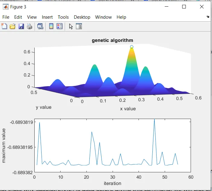
In this case we got a single optimum value.