Week 7 - Simulation of a 1D Super-sonic nozzle flow simulation using Macormack Method
Objective:-
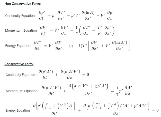
In this challenge, you are going to simulate the isentropic flow through a Quasi 1D subsonic-supersonic nozzle. You will derive both the conservation and non-conservation forms of the governing equations and solve them using MacCormack's technique.
You need to show the following plots inside your report
1. Steady-state distribution of primitive variables inside the nozzle
2. Time-wise variation of the primitive variables
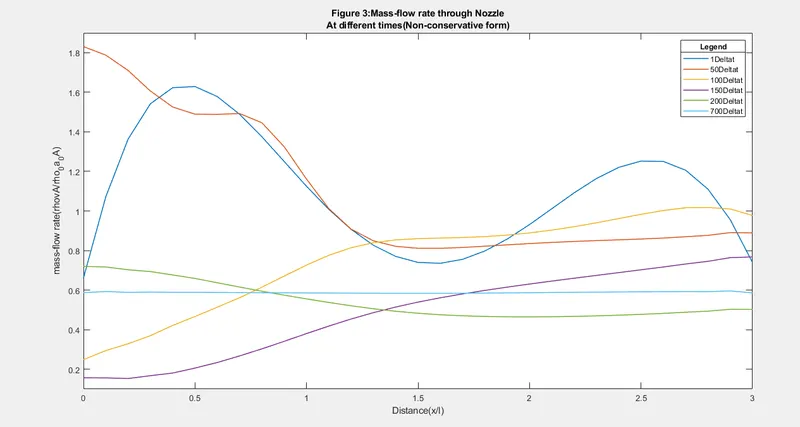
3. Variation of Mass flow rate distribution inside the nozzle at different time steps during the time-marching process
4. Comparison of Normalized mass flow rate distributions of both forms.
Solution:-
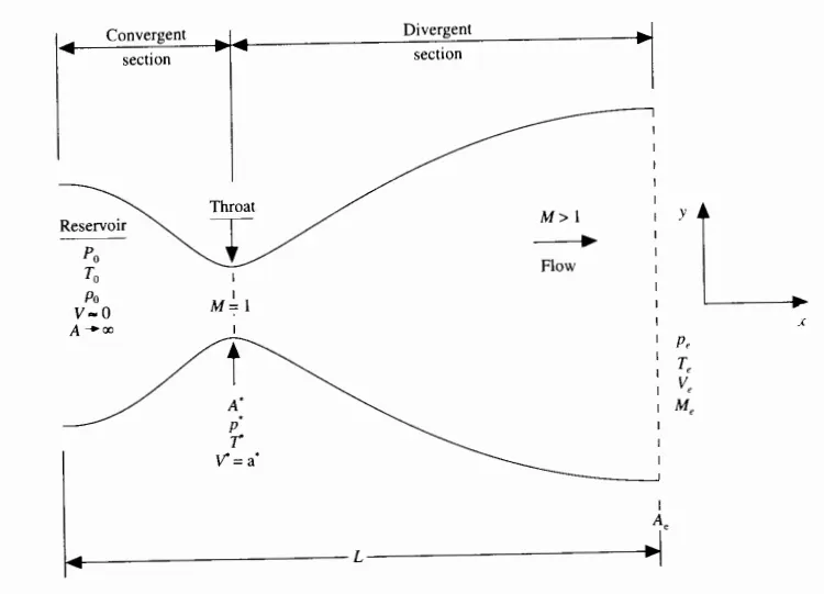
We consider the steady, isentropic flow through a convergent-divergent nozzle as sketched in Fig. The flow at the inlet to the nozzle comes from a reservoir where the pressure and temperature are denoted by p0, and To, respectively. The cross-sectional area of the reservoir is large and hence the velocity is very small. Thus, Po and T0 are the stagnation values, or total pressure and total temperature, respectively. The flow expands 1sentrop1cally. to supersonic speeds at the nozzle exit, where the exit pressure, temperature, velocity, and Mach number are denoted by Pe, Te, V, and Me, respectively. The flow is locally subsonic in the convergent section of the nozzle, some at the throat (minimum area), and supersonic at the divergent section.
Governing Eq:-
The Setup:-
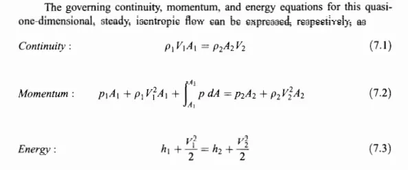
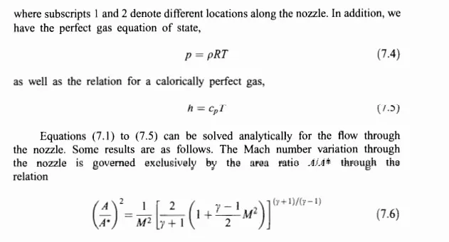
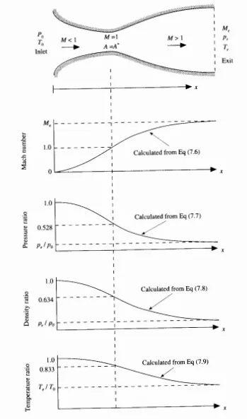
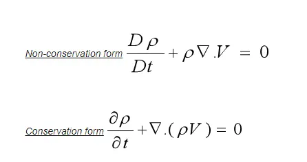
The Governing equation can be derived into two forms they are Non-conservation and Conservation.
MacCormack method:-
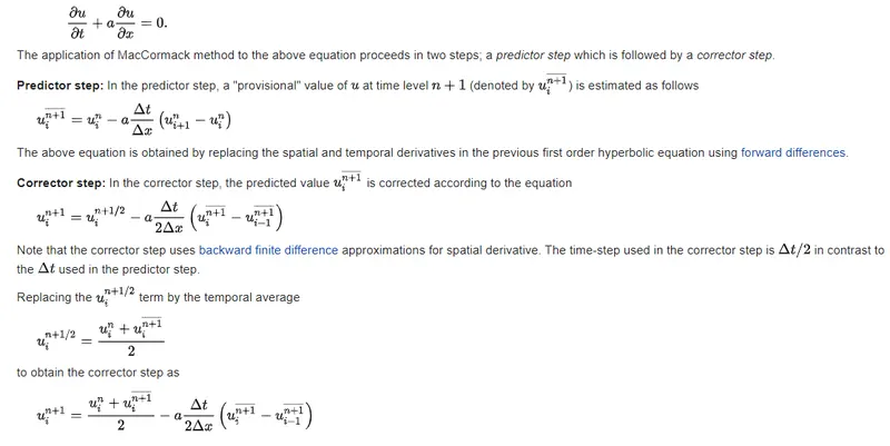
In CFD the MacCormack method is a widely used discretization scheme for the numerical solution of hyperbolic partial differential equations. This second-order finite difference method was introduced by Robert W. MacCormack in 1969.
Main program:-
The program is divided into 3 parts.First is Quasi 1D subsonic-supersonic nozzle code which is the main program followed by two sub-program 1] Non-conservation and 2] Conservation.
1] Solving 1D subsonic-supersonic nozzle problem.
%%%%%Week 7_Project_2%%%%%
clear, close all
clc

% Initializing the Domain
% inputs
L = 3;
nodes = [61,31];
for i = 1:2
 n = nodes(i);
 x = linspace(0,L,n);
 dx = x(2)-x(1);
 gamma = 1.4;
 a = 1+2.2*(x-1.5).^2; % area
 nt = 1400;
 c = 0.5; % Courant number
 throat = find(a==1);

% Solving the flow variable with Conservaion and non-conservation flow
[rho,v,t,p,rho_th,t_th,p_th,m_nc,M,M_th] = Non_conservative(x,dx,a,n,c,nt,gamma,throat);
[rho_c,v_c,t_c,p_c,rho_th_c,t_th_c,p_th_c,m_c,M_c,M_th_c] = conservative(x,dx,a,n,c,nt,gamma,throat);

% Plotting the results
figure(5)
subplot(2,2,1)
plot(rho_th,'r','linestyle','--');
hold on
grid on
plot(rho_th_c,'b');
hold off
ylabel('Non-dimensional density');
xlabel('time Step');
legend('non-conservation form','conservation form')
axis([0 1400 0 1.3]);

subplot(2,2,2);
plot(p_th,'r','linestyle','--');
hold on
plot(p_th_c,'b');
hold off
grid on
ylabel('Non-dimensional Pressure');
xlabel('time Step ');
legend('non-conservation form','conservation form')
axis([0 1400 0.4 1.1]);

subplot(2,2,3)
plot(t_th,'r','linestyle','--');
hold on
plot(t_th_c,'b');
hold off
grid on
ylabel('Non-dimensional Temperature');
xlabel('time Step ');
legend('non-conservation form','conservation form')
axis([0 1400 0.6 1]);

subplot(2,2,4);
plot(M_th,'r','linestyle','--');
hold on
plot(M_th_c,'b');
hold off
grid on
xlabel('time Step ');
ylabel('Non-dimensional Mach Number');
legend('non-conservation form','conservation form')
axis([0 1400 0.6 1.4]);
sgtitle('Figure 5:Plot showing time-wise Primitive variable inside Nozzle','Fontsize',13);

 % Plotting the P,rho,T,M wrt Nozzle length
 figure(6)
 subplot(2,2,1);
 plot(x,M,'r','marker','*');
 hold on
 plot(x,M_c,'b');
 hold off
 grid off
 xlabel('distance');
 ylabel('Non-dimensional Mach no.');
 legend('non-conservation form','conservation form')
 axis([0 3 0 4]);

 subplot(2,2,2)
 plot(x,p,'r','marker','*');
 hold on
 plot(x,p_c,'b');
 hold off
 grid off
 xlabel('distance');
 ylabel('Non-dimensional Pressure');
 legend('non-conservation form','conservation form')
 axis([0 3 0 1.01]);

 subplot(2,2,3);
 plot(x,rho,'r','marker','*');
 hold on
 plot(x,rho_c,'b');
 hold off
 grid off
 xlabel('distance');
 ylabel('Non-dimensional Density');
 legend('non-conservation form','conservation form')
 axis([0 3 0 1.01]);

 subplot(2,2,4);
 plot(x,t,'r','marker','*');
 hold on
 plot(x,t_c,'b');
 hold off
 grid off
 xlabel('distance');
 ylabel('Non-dimensional Temperature');
 legend('non-conservation form','conservation form')
 axis([0 3 0 1.01]);
 sgtitle('Figure 6:Plot showing steady state inside Nozzel','Fontsize',13')

 % mass flow rate comparison for both conservation and non-conservation form
 figure(7)
 plot(x,m_nc,'b');
 hold on
 plot(x,m_c,'r');
 % Analytical solution
 line([0 3],[0.579 0.579]);
 legend('non-conservation form','conservation form','location','best')
 leg = legend('show');
 title(leg,'legend');
 strx = sprintf('Figure 7: Steady state mass flow rate of conservation vs non-conservation=%d',n);
 title(strx,'Fontsize',12);
 xlabel('distance');
 ylabel('Non-dimensional Mass flow rate');
 hold off
end
2] Non-conservation function
% Function for Non-Conservative

function [rho,v,t,p,rho_th,t_th,p_th,m_nc,M,M_th] = Non_conservative(x,dx,a,n,c,nt,gamma,throat)

  mncplot = [1,50,100,150,200,700];

% calculate inital profiles
rho = 1-0.3146*x;
t = 1-0.2314*x; % t = temperature
v = (0.1+1.09*x).*t.^0.5;

% Outer time loop
for k = 1:nt
    rho_old = rho;
    v_old = v;
    t_old = t;

      %Time-step
    dt = min(c.*dx./((sqrt(t))+v));

    % Predictor Method
for j = 2:n-1
    dvdx = (v(j+1)-v(j))/dx;
    drhodx = (rho(j+1)-rho(j))/dx;
    dtdx = (t(j+1)-t(j))/dx;
    dlog_adx = (log(a(j+1))-log(a(j)))/dx;

    % Continuity Eqn
    drhodt_p(j) = -rho(j)*dvdx-rho(j)*v(j)*dlog_adx - v(j)*drhodx;
    % Momentum Eqn
    dvdt_p(j) = -v(j)*dvdx-(1/gamma)*(dtdx+(t(j)/rho(j))*drhodx);
   % Energy Eqn
    dtdt_p(j) = -v(j)*dtdx-(gamma-1)*t(j)*(dvdx+v(j)*dlog_adx);

    % Solution update
    rho(j) = rho(j)+drhodt_p(j)*dt;
    v(j) = v(j)+dvdt_p(j)*dt;
    t(j) = t(j)+dtdt_p(j)*dt;
end

    % Corrector Method
for j = 2:n-1
    dvdx = (v(j)-v(j-1))/dx;
    drhodx = (rho(j)-rho(j-1))/dx;
    dtdx = (t(j)-t(j-1))/dx;
    dlog_adx = (log(a(j))-log(a(j-1)))/dx;

    % Continuity Eqn
    drhodt_c(j) = -rho(j)*dvdx-rho(j)*v(j)*dlog_adx - v(j)*drhodx;

    % Momentum Eqn
    dvdt_c(j) = -v(j)*dvdx-(1/gamma)*(dtdx+(t(j)/rho(j))*drhodx);

    % Energy Eqn
    dtdt_c(j) = -v(j)*dtdx-(gamma-1)*t(j)*(dvdx+v(j)*dlog_adx);

end
     % Compute the Avg time derivative
     drhodt = 0.5*(drhodt_p + drhodt_c);
     dvdt = 0.5*(dvdt_p + dvdt_c);
     dtdt = 0.5*(dtdt_p + dtdt_c);

     % Final solution update
for i = 2:n-1
    rho(i) = rho_old(i)+ drhodt(i)*dt;
    v(i) = v_old(i)+ dvdt(i)*dt;
    t(i) = t_old(i)+ dtdt(i)*dt;
end

    % Apply Boundary Condn
    % Inlet BC
     v(1) = 2*v(2)-v(3);
     rho(1) = 1;
     t(1) = 1;
     % Outlet BC
     v(n) = 2*v(n-1)-v(n-2);
     rho(n) = 2*rho(n-1)-rho(n-2);
     t(n) = 2*t(n-1)-t(n-2);

     %  % Calculating Pressure, mach no. and mass flow rate.
     p = rho.*t;
     M = v./sqrt(t);
     m_nc = rho.*a.*v;

       % Calculating the throat section
     M_th(k)= M(throat);        % Mach No.
     rho_th(k) = rho(throat);   % Density ratio
     t_th(k) = t(throat);       % Non-dimensional temp
     p_th(k) = p(throat);       % Pressure ratio

      % Now comparing mass-flow rate with time
     for j = 1:1:6
         if k == mncplot(j)
             for s=1:1:n
                 mnc_call(s,j) = m_nc(s);
             end
         end
     end
end
     figure(3);
     plot(x,mnc_call,'linewidth',1.1);
     axis([0 3 0.1 1.9]);
     legendcell = strcat(string(mncplot(1:6)),"Deltat");
     legend(legendcell,'location','northeast');
     leg = legend('show');
     title(leg,'Legend');
     title({'Figure 3:Mass-flow rate through Nozzle';'At different times(Non-conservative form)'},'Fontsize',11)
     xlabel('Distance(x/l)');
     ylabel('mass-flow rate(rhovA/rho_0a_0A)');
end
3] Conservative Function
% Function for Conservative

function [rho_c,v_c,t_c,p_c,rho_th_c,t_th_c,p_th_c,m_c,M_c,M_th_c] = conservative(x,dx,a,n,c,nt,gamma,throat)

mcplot = [1,100,200,700];

% calculate inital profiles
for i = 1:n
      if x(i)>=0 && x(i)<0.5
        rho_c(i)=1;
        t_c(i)=1;
      elseif x(i)>=0.5 && x(i)<1.5
        rho_c(i)=1.0-(0.366*(x(i)-0.5));
        t_c(i)=1-0.167*(x(i)-0.5);
      elseif x(i)>=1.5 && x(i)<=3.0
        rho_c(i)=0.634-(0.3879*(x(i)-1.5));
        t_c(i)=0.833-(0.3507*(x(i)-1.5));
      end
end

% steady state flow
v_c = 0.59./(rho_c.*a);
p_c = rho_c.*t_c;

% Solution Vectors
U1 = rho_c.*a;
U2 = rho_c.*a.*v_c;
%U3 = U1.*((t_c./gamma-1)+(gamma/2).*(v_c.^2));
U3 = U1.*((t_c./(gamma-1))+(gamma/2).*(v_c.^2))

% Outer time loop
for k = 1:nt
    u1_old = U1;
    u2_old = U2;
    u3_old = U3;

      %Time-step
    dt = min(c*(dx./((t_c.^0.5)+v_c)));

    % Flux Vectors
    f1 = U2;
    term1 = (((gamma-1)/gamma)*(U3-((gamma/2)*((U2.^2)./U1))));
    f2 = ((U2.^2)./U1)+term1;
    f3 = ((gamma*U2.*U3)./U1)-(gamma*(gamma-1)*(U2.^3))./(2*U1.^2);

    % MacCormack Technique
         % Predictor Method
 for j = 2:n-1
    dU1dx_p = (f1(j+1)-f1(j))/dx;
    dU2dx_p = (f2(j+1)-f2(j))/dx;
    dU3dx_p = (f3(j+1)-f3(j))/dx;
    dJ2dx_p = (1/gamma)*(rho_c(j)*t_c(j))*(a(j+1)-a(j))/dx;

    % Continuity Eqn
    dU1dt_p(j) = -dU1dx_p;

    % Momentum Eqn
    dU2dt_p(j) = -dU2dx_p + dJ2dx_p;

   % Energy Eqn
    dU3dt_p(j)= -dU3dx_p;

    % Solution update
     U1(j) = U1(j)+ dU1dt_p(j)*dt;
     U2(j) = U2(j)+ dU2dt_p(j)*dt;
     U3(j) = U3(j)+ dU3dt_p(j)*dt;
 end
    % Initialize the primitive variables and flux vector
      rho_c = U1./a;
      v_c = U2./U1;
      t_c = (gamma-1)*((U3./U1)-((gamma*v_c.^2)/2));
      p_c = rho_c.*t_c;

    % "Pure" Flux terms for Corrector step
       f1 = U2;
       term2 = (((gamma-1)/gamma)*(U3-(gamma*U2.^2)./(2*U1)));
       f2 = ((U2.^2)./U1)+term2;
       f3 = ((gamma*U2.*U3)./U1)-(gamma*(gamma-1)*(U2.^3))./(2*U1.^2);

    %    Corrector Method
 for j = 2:n-1

     df1_dx = (f1(j)-f1(j-1))/dx;
     df2_dx = (f2(j)-f2(j-1))/dx;
     df3_dx = (f3(j)-f3(j-1))/dx;
     J3_dx = (1/gamma)*(rho_c(j)*t_c(j))*(a(j)-a(j-1))/dx;

       % Continuity Eqn
    dU1dt_c(j) = -df1_dx;

        % Momentum Eqn
    dU2dt_c(j) = -df2_dx+J3_dx;

        % Energy Eqn
    dU3dt_c(j)= -df3_dx;

 end
      % Compute the Avg time derivative
       dU1dt = 0.5*(dU1dt_p + dU1dt_c);
       dU2dt = 0.5*(dU2dt_p + dU2dt_c);
       dU3dt = 0.5*(dU3dt_p + dU3dt_c);

     % Final solution update
 for j = 2:n-1
     U1(j) = u1_old(j)+ dU1dt(j)*dt;
     U2(j) = u2_old(j)+ dU2dt(j)*dt;
     U3(j) = u3_old(j)+ dU3dt(j)*dt;
 end
     % Apply Boundary Condition
     % Inlet BC
     %v_c(1)= 2*U2(2)-v_c(3);
     v_c(1)= U2(1)/U1(1);
     U1(1) = a(1);
     %U2(1) = 2*U2(2)-U3(3);
     U2(1) = 2*U2(2)-U2(3);
     %U3(1) = U1(1)*(1/(gamma-1)+(0.5*gamma*v_c(1)^2));
     U3(1) = U1(1)*(t_c(1)/(gamma-1)+(0.5*gamma*v_c(1)^2))
     % Outlet BC
     U1(n) = 2*U1(n-1) - U1(n-2);
     U2(n) = 2*U2(n-1) - U2(n-2);
     U3(n) = 2*U3(n-1) - U3(n-2);

     % Initialize the primitive variables .
     rho_c = U1./a;
     v_c = U2./U1;
     %t_c = (gamma-1)*(U3/U1)-((gamma/2)*v_c.^2);
     t_c = (gamma-1)*((U3/U1)-(gamma/2)*v_c.^2)
     p_c = rho_c.*t_c;

     % Calculating Pressure, mach no. and mass flow rate.
     M_c = v_c./sqrt(t_c);
     m_c = rho_c.*a.*v_c;

     % Calculating the throat section
     M_th_c(k)= M_c(throat);        % Mach No.
     rho_th_c(k) = rho_c(throat);   % Density ratio
     t_th_c(k) = t_c(throat);       % Non-dimensional temp
     p_th_c(k) = p_c(throat);       % Pressure ratio

     % Now comparing mass-flow rate with time
     for j = 1:1:4
         if k == mcplot(j)
             for s=1:1:n
                 mc_call(s,j) = m_c(s);
             end
         end
     end
end
     figure(4);
     plot(x,mc_call,'linewidth',1.0);
     axis([0 3 0.5 0.7]);
     legendcell = strcat(string(mcplot(1:4)),"Deltat");
     legend(legendcell,'location','northeast');
     leg = legend('show');
     title(leg,'Legend');
     title({'Figure 4:Mass-flow rate through Nozzle';'At different times(conservative form)'},'Fontsize',11)
     xlabel('Distance(x/l)');
     ylabel('mass-flow rate(rhovA/rho_0a_0A)');

end
Code Explanation:-
- We have started our code with Close all, clear, clc. This commands help us in clearing the backlog data, clears the command window.
- After that we have to assign the input parameters to the code eg.x,dx,l,etc.
- Tic-Toc commands are used to calculate the time betwwen two functions, Then the functions which we have created, which are the Non-conservative and conservative with there neccessary inputs are given to them.
- After that plotting is done,1] Plotting the P,rho,T,M wrt Nozzle length, 2] Mass flow rate comparison for both conservation and non-conservation form.
- Then Analytical solution is calculated.
- Now moving now to the function for Non-Conservative code
- First we have to create the function, give correct input parameters to it
- the calculating the initial profiles and then doing the Predictor and corrector method.In it we have calculate the mass flow rate, Pressurre,Density,velocity,Temperature,etc.
- For initial profile,for loop is used with else-if commands.
- Now outer Time loop is formed, in this the predictor method and corrector method are used, which is the maccormack method.
- After that updating the solution with old values.so that old values will be considered.
- After that applying the Boundary condition within the foor loop and calculating the values ofthroat sectio.
- Then the plloting is done for x(distance) and mass flow rate and then END.
- Now moving now to the function for Conservative code
- First we have to create the function, give correct input parameters to it
- the calculating the initial profiles and then doing the Predictor and corrector method.In it we have calculate the mach no. mass flow rate, Pressurre,Density,velocity,Temperature,etc.
- For initial profile,for loop is used with else-if commands.
- Now outer Time loop is formed, in this the predictor method and corrector method are used, which is the maccormack method.
- After that updating the solution with old values.so that old values will be considered.
- After that applying the Boundary condition within the foor loop and calculating the values ofthroat sectio.
- Then the plloting is done for x(distance) and mass flow rate and then END.
Plots
1] Mass flow rate through nozzle at different times(Non-conservative form)
Observation
here we can see after 450 time-steps the solution starts to become stable and after that attaining the constant value
2] Mass flow rate through nozzle at different times, conservative form
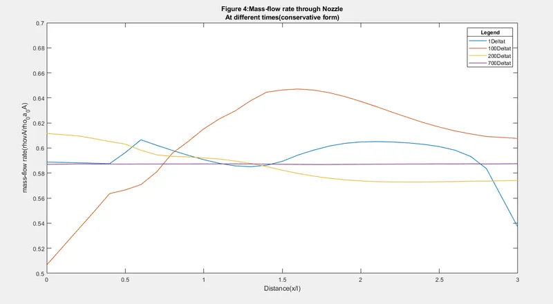
Observation
here we can see after 450 time-steps the solution starts to become stable and after that attaining the constant value
3] Time-wise primitive variables inside nozzle
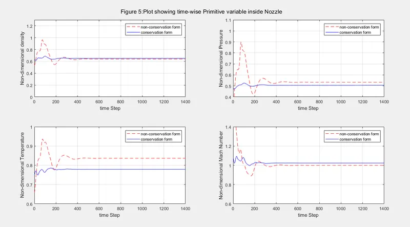
Observation
From the above plots we can see that the primitive variables the non-conservative form starts at higher rate but acheives stable solution after cretain period.
4] Steady staedy inside nozzel
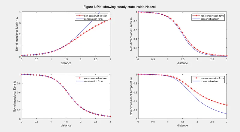
Observation
Here we can see that, both the forms are giving nearly same solution.
5] Steady state mass flow rate of conservative vs Non-conservative.
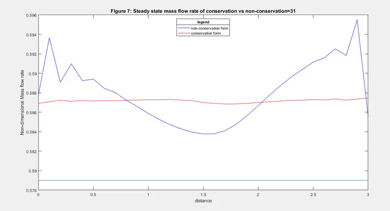
Observation
Her we can see that the non-conservative form has higher oscillation than the conservative part. So the conservative form achieves statbility faster thane the non-conservative form in lesser time period.
Grid dependency
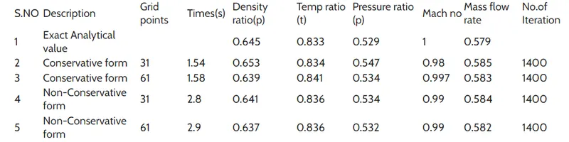
As we can cleary see that both the form have sligth difference in them its just that the conservative form attains the stability faster and its more accurate then the non-conservative form.