Week 5 - Mid term project - Solving the steady and unsteady 2D heat conduction problem
Steady state analysis
Objective:- Steady state analysis & Transient State Analysis using Solve the 2D heat conduction equation by using the point iterative techniques and use the following methods for solving implicit equations.
1. Jacobi
2. Gauss-seidel
3. Successive over-relaxation
Your absolute error criteria is 1e-4
Solution: -
`->` The steady state 2D heat conduction eq
`(del^2T)/(dx^2)+(del^2T)/(dy^2)`
After discritizing it we get
`Tp = 1/k ((Tl+Tr)/(Deltax^2))+1/k((Tt+Tb)/(Deltay^2))`
Now we start solving steady state using iterative method as the boundary cond. are already given to us now we can start the coding for steady state, the code is given below
clear;
close all
clc
% Inputs
% grid points along X-axis and Y-axis.
nx = 10;
ny = nx;
L = 10; % Length of the domain
 x = linspace(0,L,nx) ;
 y = linspace(0,L,ny);
 dx = L/(nx-1);
 dy = L/(ny-1);

 A = 1.4; % ALPHA value

% Applying BC
T_L = 400;
T_R = 800;
T_T = 600;
T_B = 900;
T = ones(nx,ny);
T(:,1) =T_L;
T(:,10) = T_R;
T(1,:) = T_T;
T(10,:) = T_B;
 tol = 1e-4;
Told = T;
Tinitial =  T;
[X,Y] = meshgrid(x,y);
error = 9e9;
iter = 0;

for iterative_solver =1:3
    while (error>tol)
        for i = 2:nx-1
        for j = 2:ny-1
            if(iterative_solver ==1)
%
                T(i,j) = Jacobi_iter(Told,i,j);
%                      Jacobi_iter = 1;
            elseif (iterative_solver ==2)
%
                T(i,j) = GS_iter(T,i,j);
%                     GS_iter = 1;
            elseif(iterative_solver ==3)
%
                T(i,j) = SOR_iter(T,Told,i,j,A);
%                     SOR_iter = 1;
            end

        end
        end
        error = max(max(abs(Told-T)));
          iter = iter+1;
            Told = T;

            % Plotting
       if(iterative_solver ==1)
       figure(1)
        contourf(T);
         colormap(hsv)
        colorbar;
        axis ij;
        xlabel('x-axis')
        ylabel('y-axis')
        title_text = sprintf('Jacobi: Iteration number = %d', iter);
        title(title_text)
        pause = 0.03;
      elseif (iterative_solver ==2)
        figure(2)
        contourf(T);
         colormap(hsv)
        colorbar;
        axis ij;
        xlabel('x-axis')
        ylabel('y-axis')
        title_text = sprintf('Gauss: Iteration number = %d', iter);
        title(title_text)
        pause = 0.03;
      elseif(iterative_solver ==3)

        figure(3)
        contourf(T);
        colorbar;
        colormap(hsv)
        axis ij;
        xlabel('x-axis')
        ylabel('y-axis')
        title_text = sprintf('SOR: Itration number = %d',iter);
        title(title_text)
        pause = 0.03;
       end


    end

    T = Tinitial;
    Told = Tinitial;
    error = 1;
    iter = 0;

end
Function for Jacobi solver
function out = Jacobi_iter(Told,i,j)

         out= 0.25*(Told(i+1,j)+Told(i-1,j)+Told(i,j+1)+Told(i,j-1));
end
Function for GS - solver
function out = GS_iter(T,i,j)
        out = 0.25*(T(i+1,j)+T(i-1,j)+T(i,j+1)+T(i,j-1));
end
Function for SOR-Solver
function out = SOR_iter(T,Told,i,j,A)
        out =(1-A)*Told(i,j)+ (A*0.25*(T(i,j-1)+Told(i,j+1)+T(i-1,j)+Told(i+1,j)));
end
In the above code at first we have to give all the Inputs which are requrid for the problem which are defining the boundary cond. ,length of the domain, number of nords along X & Y directon and creating a grid,etc and here i have created function for the iterative solvers like jacobi , gauss sidel & SOR method the function codes are given below the main code adter defining the functions the we have define them into our main code in others words calling then in different code which is called as calling the function code . After giving all he inputs to our code no we have to use the iterative solver method which consists of time loop and space loop which are the important factors of our code this were the iteration takes place and we have to use this same method on jacobi and same follows other iterative methods and writing the code for displaying the output we have plot the results to check the solution is right or worng other words at what point it is getting converged so we have to plot the results in side the while loop so we can see the animation like how it gets converged that is also given in the above code same is to done for the other iterative menthods results of this methods are given below
Output :- (1) Results Jacobi iterative-solver
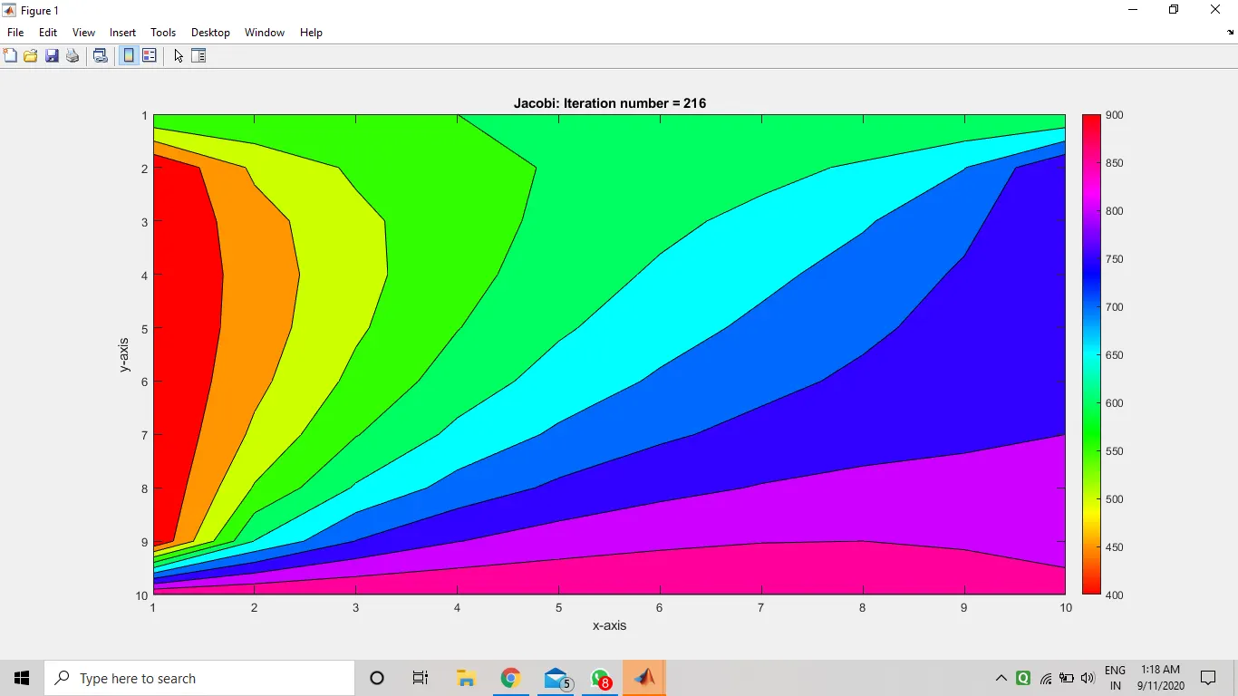
As we can see jacobi method has take 216 iterations to solve for steady state the color distribution are the temperature at location, As jacobi use old time step thats why it takes more number of iteration to solve the problem and also it takes more time than compared to other two methods.
(2)Results GS-iterative-solver
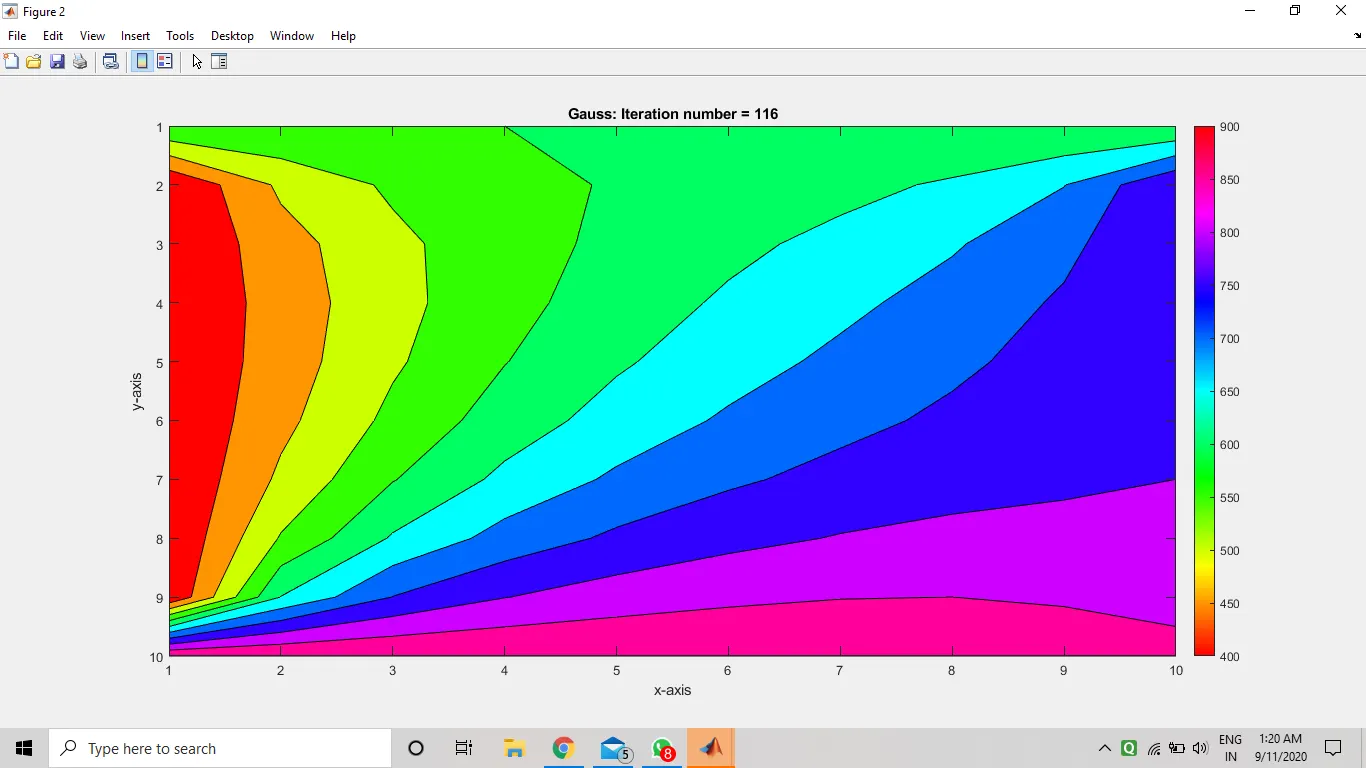
GS takes less number of iteration and less time than the jacobi method as in this we use the new calculated value of the time step into the next iteration so we can see only 166 iterations are to converge the eq
(3)Results SOR iterative-solver
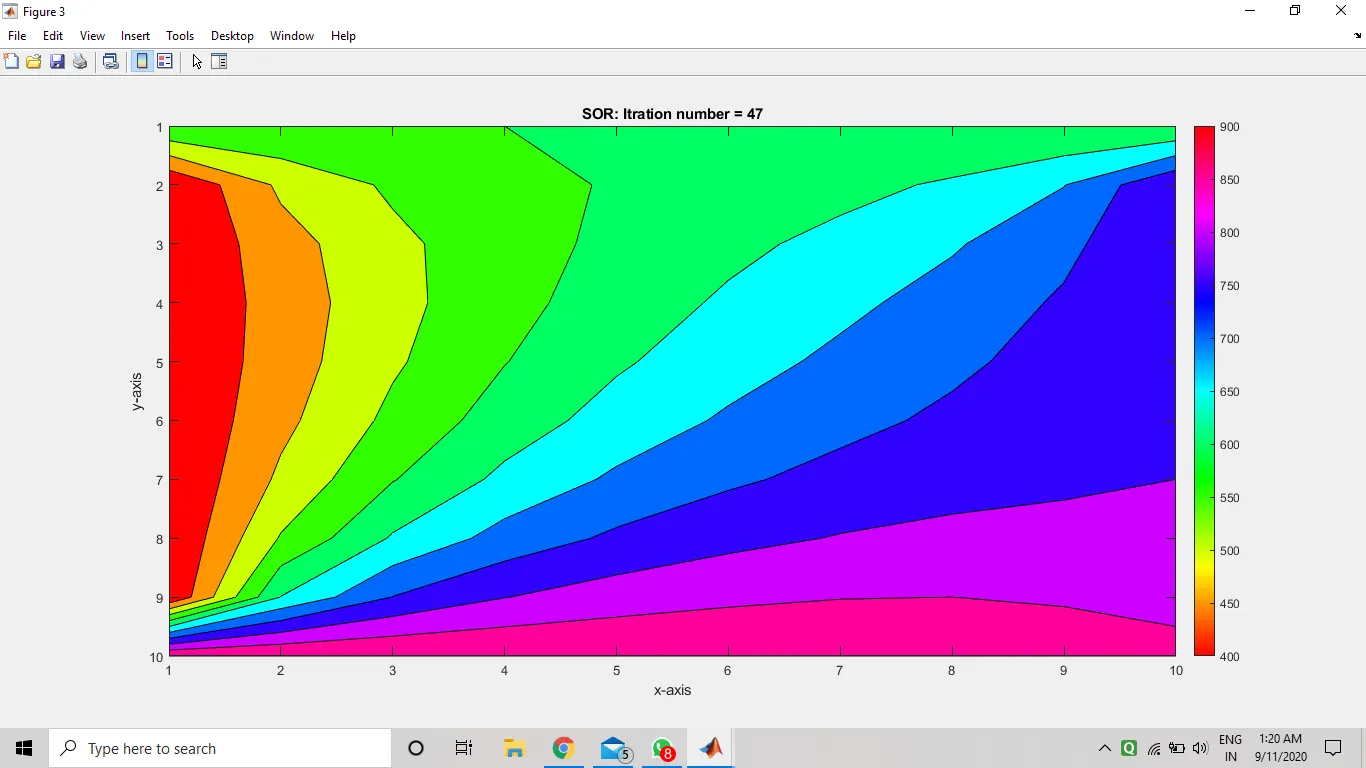
This solver has only taken 47 iteration to converge the eq this eq. is called as Successive over-relaxation(SOR) it takes less time than the other two methods as this the advance iteration solver using the alpha value in it, convergence is higher in SOR than other two values
----------------------------------------------------------------------------------------------------------------------------------------------------------------------------------------------------------------
Transient State Analysis
`->` In Transient state/Unsteady state the temperature changes with time and conveges to steady state.Transient state/Unsteady state in this we have use both the methods which are Implicit and Explicit schemes
Explicit schemes
`(delT)/(delt)+alpha*Delta(T)`
after solving this eq we get
`T^(n+1) (i,j) = T^n(i,j)+alpha*DeltaT((Tr-2Tp+Tl)/(Deltax^2)+(Tt-2Tp+Tb)/(Deltay^2))`
clear;
close all
clc
% Inputs
% grid points along X-axis and Y-axis.
nx = 10;
ny = nx;
L = 10; % Length of the domain
 x = linspace(0,L,nx) ;
 y = linspace(0,L,ny);
 dx = L/(nx-1);
 dy = L/(ny-1);

 A = 1.5; % ALPHA value

% Applying BC
T_L = 400;
T_R = 800;
T_T = 600;
T_B = 900;
T = ones(nx,ny);
T(:,1) =T_L;
T(:,10) = T_R;
T(1,:) = T_T;
T(10,:) = T_B;
dt = 0.01;
k1 = A*dt/(dx^2);
k2 = A*dt/(dy^2);
 tol = 1e-4;
 Told  = T;
Tprev = T;
[X,Y] = meshgrid(x,y);
error = 9e9;
iter = 0;

% iter = 1;
   while error>tol
        for i = 2:nx-1
        for j = 2:ny-1
            T(i,j) = (1-2*k1-2*k2)*Tprev(i,j)+ k1*(Tprev(i-1,j)+Tprev(i+1,j))+k2*(Tprev(i,j+1)+Tprev(i,j-1));

        end
        end

          error = max(max(abs(Tprev-T)));
           iter = iter+1;
           Tprev = T;

         figure(1)
        contourf(T);
        set(gca,'YDIR','reverse');
        colormap(hsv)
        colorbar;
        axis ij;
        xlabel('x-axis')
        ylabel('y-axis')
        title_text = sprintf('Jacobi iter = %d',iter);
        title(title_text)
        pause = 0.003;

   end
In this code we already know most of these which were used in the steady state only k1 and k2 values are added and chnage in formula and like steady state we must write the code in the while loop other wise it wont run the results are given below
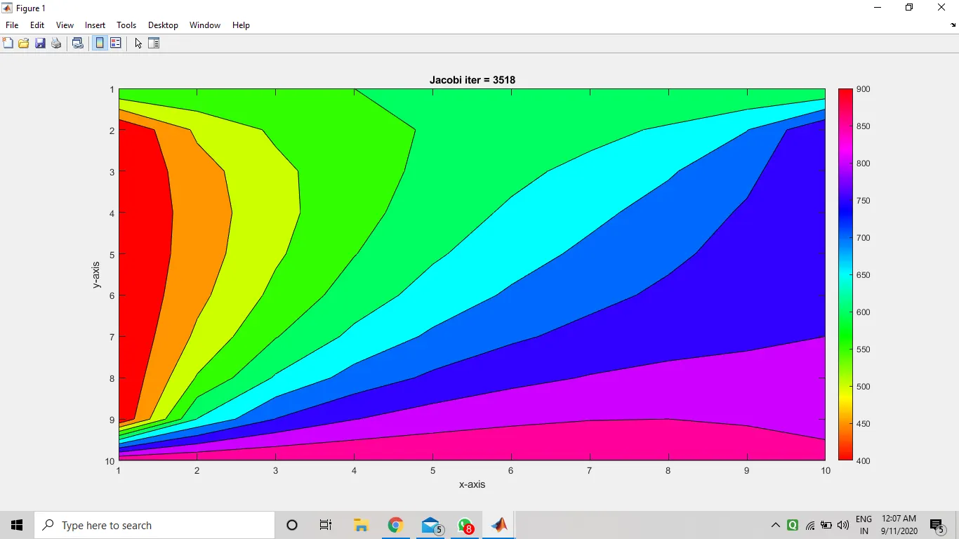
As it can be seen the time and iteration taken by this method is to high and iteraton taken to converge is 3518 and the CFL value is 0.0121
Implicit method
for this method we just have to use our iterative solver just like we did in the steady state the code for it is given below
% Solving unsteady state by Implicit method
%Inputs

clear;
close all
clc
% Inputs
% grid points along X-axis and Y-axis.
nx = 10;
ny = nx;
L = 10; % Length of the domain
 x = linspace(0,L,nx) ;
 y = linspace(0,L,ny);
 dx = L/(nx-1);
 dy = L/(ny-1);

 A = 1.4; % ALPHA value

% Applying BC
T_L = 400;
T_R = 800;
T_T = 600;
T_B = 900;
T = ones(nx,ny);
T(:,1) =T_L;
T(:,10) = T_R;
T(1,:) = T_T;
T(10,:) = T_B;
dt = 1.4;
k1 = A*dt/(dx^2);
k2 = A*dt/(dy^2);
 tol = 1e-4;
 Told  = T;
 Tinitial = T;
[X,Y] = meshgrid(x,y);
error = 9e9;
iter = 0;
Tprev = T;
                            % Solving Jacobi iter EQ


for nt = 1:1000
 error = 1;
    while error>tol
        for i = 2:nx-1
            for j = 2:ny-1
                term1 = (1+(2*k1)+(2*k2))^-1;
                term2 = k1*term1;
                term3 = k2*term1;
                H = (Told(i-1,j)+Told(i+1,j));
                V = (Told(i,j-1)+Told(i,j+1));
                T(i,j) = (term1*(Tprev(i,j))+term2*H+term3*V);

            end
        end
        error = max(max(abs(Told-T)));
         iter = iter+1;
        Told = T;


          figure(1)
        contourf(T);
        set(gca,'YDIR','reverse');
         colormap(hsv)
        colorbar;
        axis ij;
        xlabel('x-axis')
        ylabel('y-axis')
        title_text = sprintf('Jacobi: Iteration number = %d', iter);
        title(title_text)
        pause = 0.03;


    end
    Tprev  = T;
%      T = Tinitial;
%     Told = Tinitial;
%     error = 1;
%     iter = 0;

 end


T = Tinitial;
T_prev = Tinitial;


                            % Solving GS iter EQ

for k = 1:nt
    error = 1;
    while error>tol
        for i = 2:nx-1
            for j = 2:ny-1
                term1 = (1+(2*k1)+(2*k2))^-1;
                term2 = k1*term1;
                term3 = k2*term1;
                H = (T(i-1,j)+T(i+1,j));
                V = (T(i,j-1)+T(i,j+1));
                T(i,j) = (term1*(Tprev(i,j))+(term2*H)+(term3*V));

            end
        end
        error = max(abs(Told-T));
       Told = T;
        iter = iter+1;


         figure(2)
        contourf(T);
         colormap(hsv)
        colorbar;
        axis ij;
        xlabel('x-axis')
        ylabel('y-axis')
        title_text = sprintf('GS: Iteration number = %d', iter);
        title(title_text)
        pause = 0.03;


    end
    Tprev  = T;
    error = 1;
end


T = Tinitial;
T_old = Tinitial;
                            % Solving SOR iter EQ

for k = 1:nt
    error = 1;
     while error>tol
        for i = 2:nx-1
            for j = 2:ny-1
                term1 = (1+(2*k1)+(2*k2))^-1;
                term2 = k1*term1;
                term3 = k2*term1;
                H = (Told(i-1,j)+Told(i+1,j));
                V = (T(i,j-1)+Told(i,j+1));
                T(i,j) = (1-A)*Told(i,j)+A*(term1*(Tprev(i,j))+(term2*H)+(term3*V));

            end
        end

        error = max(abs(Told-T));
       Told = T;
        iter = iter+1;


         figure(3)
        contourf(T);
         colormap(hsv)
        colorbar;
        axis ij;
        xlabel('x-axis')
        ylabel('y-axis')
        title_text = sprintf('SOR: Iteration number = %d', iter);
        title(title_text)
        pause = 0.03;


    end

    Tprev  = T;

T = Tinitial;
T_old = Tinitial;
error = 1;
end
its the same like we did in the other methods we just interested the results of the this solvers
Outputs/Results :- (1) Jacobi-iter
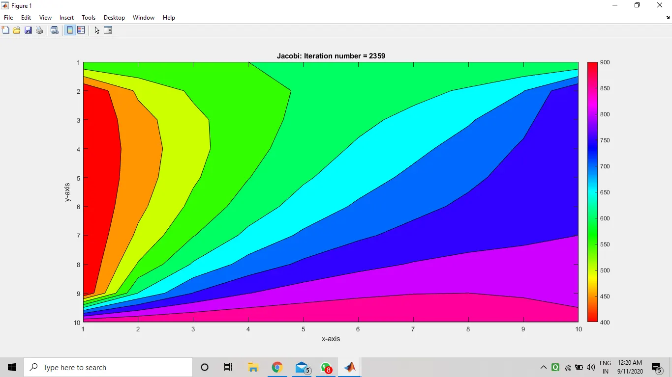
As you can see jacobi has taken 2359 iteration to get converge as we are doing ig for unsteady state its takes time to converge
(2) GS-iter
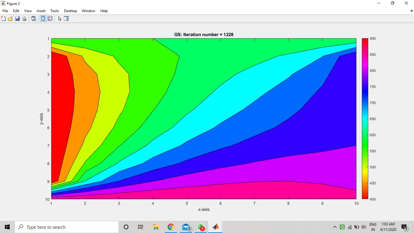
GS method has taken 1228 iteration to solve the unsteady state as it is better than the jacobi method as we already know GS uses the new value and not the old time step value
(3) SOR - iter
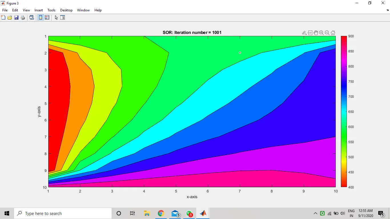
As we can see already in just 1001 iteration values the figure is converged which is far better than the other two methods
As we have already seen in both the condn which are steady and unsteady state SOR method has been far better than other two methods beause it is fast and less time taking