Week 4 - Genetic Algorithm

Objective:-

• Try to understand the concept of the genetic algorithm by referring to various sources before you attend this challenge. Look out for information regarding the stalagmite function and ways to optimize it.
• Write a code in MATLAB to optimize the stalagmite function and find the global maxima of the function.
• Clearly explain the concept of genetic algorithm in your own words and also explain the syntax for ga in MATLAB in your report.
• Make sure that your code gives the same output, even if it is made to run several times.
• Plot graphs for all 3 studies and for F maximum vs no. of iterations. Title and axes labels are a must, legends could be shown if necessary.

Solution:-

1. What is Stalagmite?

`->` A stalagmite is an upward-growing mound of mineral deposits that have precipitated from water dripping onto the floor of a cave.

2. what is a Genetic algorithm?

`->` A genetic algorithm is a search heuristic that is inspired by Charles Darwin's theory of natural evolution. This algorithm reflects the process of natural selection where the fittest individuals are selected for reproduction in order to produce offspring of the next generation. A genetic algorithm (GA) is a search-based optimization technique based on the principles of Genetics and Natural Selection. It is frequently used to find optimal or near-optimal solutions to difficult problems that otherwise would take a lifetime to solve. It is frequently used to solve optimization problems

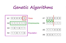
Genetic Algorithm optimization starts with population initialization, Population is the number of sample data points taken to perform the genetic algorithm operation. These sample data points undergo the following in these three steps,

1. Selection - In this step, the parents are selected from the sample data points, the main objective of the selection process is to select the highly fit individuals.
2. Cross-Over - Crossover is the most significant phase in a genetic algorithm. For each pair of parents to be mated, a crossover point is chosen at random from within the genes Offspring are created by exchanging the genes of parents among themselves until the crossover point is reached.
3. Mutation - In certain new offspring formed, some of their genes can be subjected to a mutation with a low random probability. This implies that some of the bits in the bit string can be flipped.Mutation occurs to maintain diversity within the population and prevent premature convergence.

• syntax for GA

x = ga(fun,nvars)

x = ga(fun,nvars,A,b)

x = ga(fun,nvars,A,b,Aeq,beq)

x = ga(fun,nvars,A,b,Aeq,beq,lb,ub)

x = ga(fun,nvars,A,b,Aeq,beq,lb,ub,nonlcon)

x = ga(fun,nvars,A,b,Aeq,beq,lb,ub,nonlcon,options)

x = ga(fun,nvars,A,b,[],[],lb,ub,nonlcon,IntCon)

x = ga(fun,nvars,A,b,[],[],lb,ub,nonlcon,IntCon,options)

x = ga(problem)

[x,fval] = ga(___)

[x,fval,exitflag,output] = ga(___)

[x,fval,exitflag,output,population,scores] = ga(___)

• Description of input variables

x = ga(fun,nvars) finds a local unconstrained minimum, x, to the objective function, fun. nvars is the dimension (number of design variables) of fun.

x = ga(fun,nvars,A,b) finds a local minimum x to fun, subject to the linear inequalities A*x ≤ b. ga evaluates the matrix product A*x as if x is transposed (A*x').

x = ga(fun,nvars,A,b,Aeq,beq) finds a local minimum x to fun, subject to the linear equalities Aeq*x = beq and A*x ≤ b. (Set A=[] and b=[] if no linear inequalities exist.) ga evaluates the matrix product Aeq*x as if x is transposed (Aeq*x').

x = ga(fun,nvars,A,b,Aeq,beq,lb,ub) defines a set of lower and upper bounds on the design variables, x, so that a solution is found in the range lb ≤ x ≤ ub. (Set Aeq=[] and beq=[] if no linear equalities exist.)

x = ga(fun,nvars,A,b,Aeq,beq,lb,ub,nonlcon) subjects the minimization to the constraints defined in nonlcon. The function nonlcon accepts x and returns vectors C and Ceq, representing the nonlinear inequalities and equalities respectively. ga minimizes the fun such that C(x) ≤ 0 and Ceq(x) = 0. (Set lb=[] and ub=[] if no bounds exist.)

x = ga(fun,nvars,A,b,Aeq,beq,lb,ub,nonlcon,options) minimizes with the default optimization parameters replaced by values in options. (Set nonlcon=[] if no nonlinear constraints exist.) Create options using optimoptions.

x = ga(fun,nvars,A,b,[],[],lb,ub,nonlcon,IntCon) or x = ga(fun,nvars,A,b,[],[],lb,ub,nonlcon,IntCon,options) requires that the variables listed in IntCon take integer values.

x = ga(problem) finds the minimum for problem, a structure described in problem.

[x,fval] = ga(___), for any previous input arguments, also returns fval, the value of the fitness function at x.

[x,fval,exitflag,output] = ga(___) also returns exitflag, an integer identifying the reason the algorithm terminated, and output, a structure that contains output from each generation and other information about the performance of the algorithm.

[x,fval,exitflag,output,population,scores] = ga(___) also returns a matrix population, whose rows are the final population, and a vector scores, the scores of the final population.

• Code in MATLAB to optimize the stalagmite function

clear 
close all
clc
% Gobal Optimization Prob
% Stalagmite Model

% Defining search space
x = linspace(0,0.6,150);
y = linspace(0,0.6,150);

% Creating two dim. space

[XX,YY] = meshgrid(x,y);

% Evaluating the stalagmit function.

for i = 1:length(x)
    for j = 1:length(y)
        input_vector(1) = XX(i,j);
        input_vector(2) = YY(i,j);
        f(i,j) = stalagmite(input_vector);
    end
     
end

So let us start the code with Clear all, close all, clc to start new script without cache, closing figure if it's open, and clearing the command window so we can start afresh script, To solve the global optimization problem first we have to define the search space using linspace command on x and y, what linspace command does is it will create 150 values between the 0-0.6 and then creating a two dim. space using mesh grid command, Now that we have a two dim. space to work on, the next is to Evaluating the stalagmite function for that we have to use "FOR LOOP". In this, we have to use the stalagmite function and code of this given below

function f = stalagmite(input_vector)
        x = input_vector(1);
        y = input_vector(2); 
        f1= (sin(5.1*pi*x+0.5))^6;
        f2= (sin(5.1*pi*y+0.5))^6;
        f3 = exp(((-4)*log(2)*(x-0.0067)^2)/0.64);
        f4 = exp(((-4)*log(2)*(y-0.0067)^2)/0.64);
        f = -(f1*f2*f3*f4);     
end

In the code above we can see the stalagmite function, Now as we have to perform the genetic Algorithm optimization for the stalagmite function, it requires two inputs X & Y

In the above code, we can see we have created

Now let's look at the first case which is CASE-1:- STATISTICAL BEHAVIOUR(UNBOUNDED). The code for the first case is given below.

% Case study-1 STATISTICAL BEHAVIOUR(UNBOUNDED)
num_case = 50;
tic
for i = 1:num_case
  [results ,fval(i)]= ga(@stalagmite,2);
  xval(i) = results(1);
  yval(i) = results(2);
end
study_time = toc;
figure(1)
subplot(2,1,1)
surfc(x,y,-f)
shading interp
xlabel('xlabel');
ylabel('ylabel');
hold on
plot3(xval,yval,-fval,'marker','o','markersize',5,'markerfacecolor','r')
title('UNBOUNDED')
subplot(2,1,2)
plot(-fval)
xlabel('iteration')
ylabel(' function maximum')
legend('iteration','function maximum')

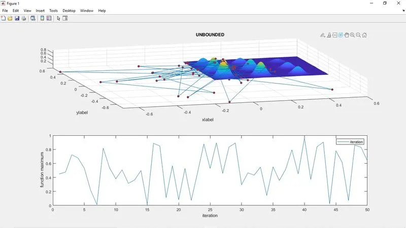
In the first case, we want to check the STATISTICAL BEHAVIOUR which is unbounded which means we are not using any bounds (upper and lower bounds) in this case. Now we will run the case(code) for 50 times, so we are using num_case=50 in the code; Now by using "FOR LOOP" we can get the outputs as we have to calculate the GA, we can use the Stalagmite function which we have created inside this "for loop", as shown in above code first using the inbuilt function ga and calling the stalagmite function using function handle. To keep the track of the time we are using the tic-toc command and then we are using the subplot command to get two plots in a single plot, using "surfc" command we can create a three-dimensional surface plot with a contour plot and after that providing other commands like title, xlabel-ylabel, legend, etc to the code.

CASE-2:- STATISTICAL BEHAVIOUR(BOUNDED) USING UPPER AND LOWER BOUNDS.

%% Case study-2 STATISTICAL BEHAVIOUR(BOUNDED) DEFINING THE UPPER AND LOWER BOUND
num_case = 50;
tic
for i = 1:num_case
  [results ,fval(i)]= ga(@stalagmite,2,[],[],[],[],[0;0],[0.4;0.4]); %x = ga(fun,nvars,A,b,Aeq,beq,lb,ub)
  xval(i) = results(1);
  yval(i) = results(2);
end
study_time_2 = toc;
figure(2)
subplot(2,1,1)
surfc(x,y,-f)
shading interp
xlabel('xlabel');
ylabel('ylabel');
hold on
plot3(xval,yval,-fval,'marker','o','markersize',5,'markerfacecolor','r')
subplot(2,1,2)
plot(-fval)
title('BOUNDED')
xlabel('iteration')
ylabel(' function maximum')
legend('iteration','function maximum')

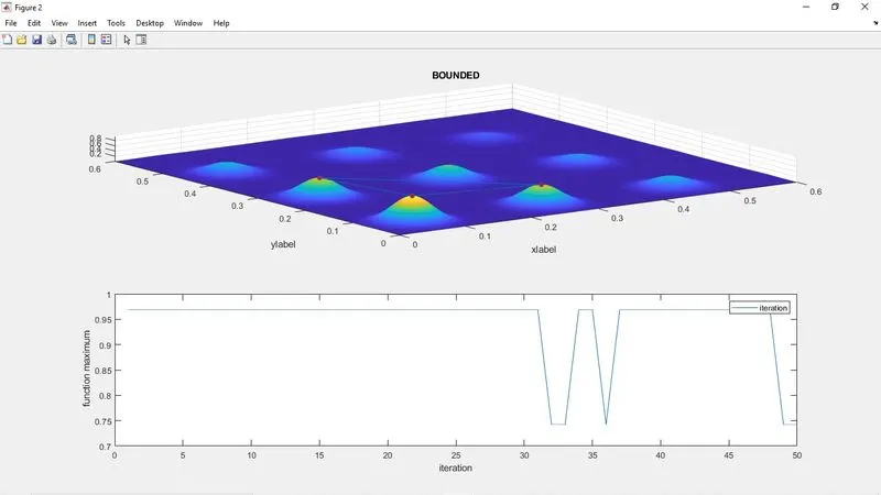
In the second case, we want to check the STATISTICAL BEHAVIOUR which is bounded which means we are using bounds (upper and lower bounds) in this case. Now we will run the case(code) for 50 times with bounds added to the code, Using the Syntax of GA( x = ga(fun,nvars,A,b,Aeq,beq,lb,ub) defines a set of lower and upper bounds on the design variables, x so that a solution is found in the range lb ≤ x ≤ ub,Set Aeq=[] and beq=[] if no linear equalities exist) we will add constraints to the ga and bounds will be [0;0] &[0.4;0.4] This helps us to improve the optimization of x and plotting is same as the first case. The case-2 showed better results than case 1.

CASE-3:- STATISTICAL BEHAVIOUR(INCREASING GA ITERATION).

%% Case study-3 STATISTICAL BEHAVIOUR(INCREASING GA ITERATION)
options = optimoptions('ga');
options = optimoptions(options,'populationsize',170);
num_case = 150;
tic
for i = 1:num_case
  [results ,fval(i)]= ga(@stalagmite,2,[],[],[],[],[0;0],[0.4;0.4],[],[],options); 
  xval(i) = results(1);
  yval(i) = results(2);
end
study_time_3 = toc;
figure(3)
subplot(2,1,1)
surfc(x,y,-f)
shading interp
xlabel('xlabel');
ylabel('ylabel');
hold on
plot3(xval,yval,-fval,'marker','o','markersize',5,'markerfacecolor','r')
subplot(2,1,2)
plot(-fval)
title('INCREASING GA ITERATION')
xlabel('iteration')
ylabel(' function maximum')
legend('iteration','function maximum')

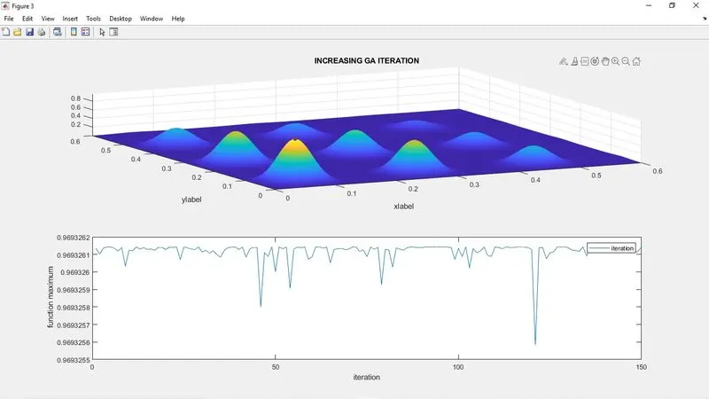
In the third case other than upper and lower bounds we are using one more constrain which is "options". The main motive of using 'option' here is to increase the population size. Increasing the population size results in better optimum values it helps to achieve the global maxima faster.

OUTPUTS OF THE CASES

CASE-1 UNBOUNDED

case-2 WITH UPPER AND LOWER BOUND

case-3 INCREASING GA ITERATION

Errors while programming

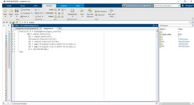
1] Providing 2-D values in the function, here we just have to provide x & y of search space, not the 2-D as we are giving this values as the input vector(1)& input vector(2) and using it in next ga minima formula.So to correct this mistake, I changed the variable to x & y as we are taking x & y in the formula

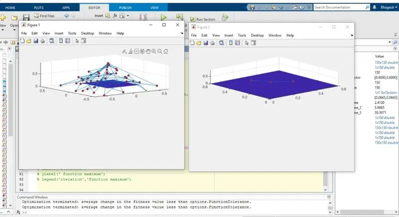
2] In the second error the Evaluating the stalagmite function went wrong because while coding, I used stalagmite function after the j- loop, to correct this error, I just used the function inside the j-loop .

references

1] https://skill-lync.com/knowledgebase/genetic-algorithm-explained

2] https://mech.iitm.ac.in/nspch52.pdf

3] https://www.tutorialspoint.com/genetic_algorithms/genetic_algorithms_introduction.htm

4] https://en.wikipedia.org/wiki/Genetic_algorithm