Week 3 - Taylor table method and Matlab code

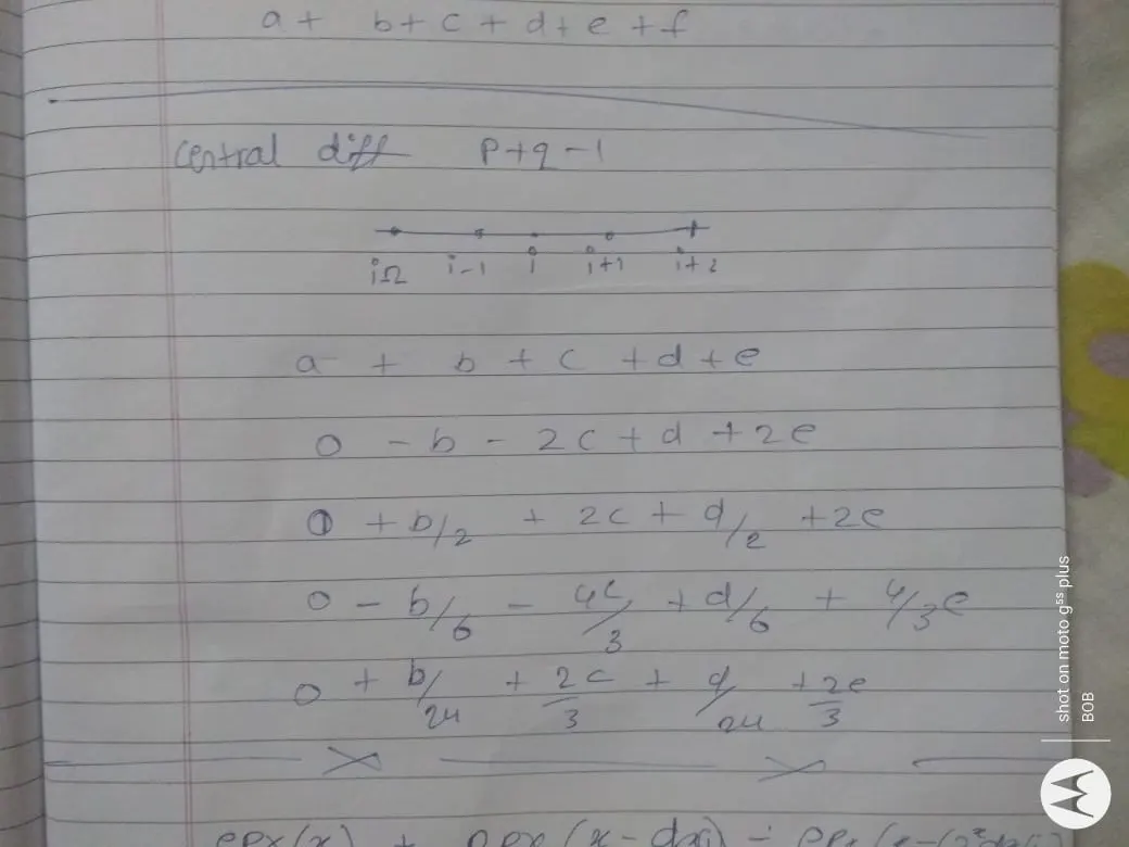
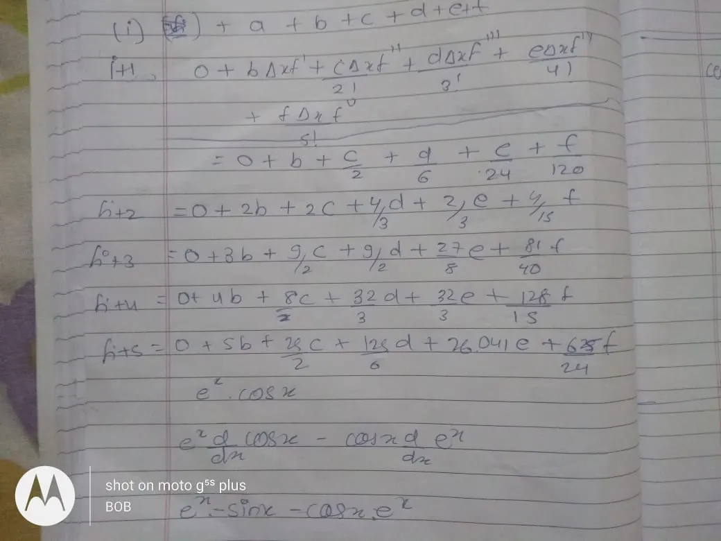
`->`As it is asked to calculate 4th order approximations of the second-order derivative for central difference ,rigth-sided difference and left -sided difference we have to calculate it by using taylor table after that we have solve the second-order derivative of the analytical function exp(x)*cos(x) photos of this approximations and the analytical derivative are given below

analytical derivative = (-2)*exp(x)*sin(x).

`->` For central difference

`->`For rigth-sided difference

`->`For left sided difference

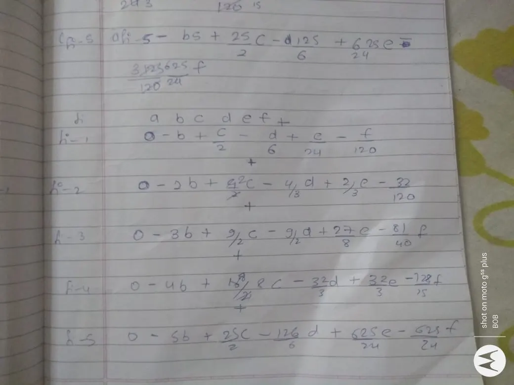
After seeing above pictures you have got the idea what are the taylor terms looks like after writing down this equations and this equations are solved by using the matrix inversion method in Matlab to obtain the coefficients because we have to covert the equations into the code as we have to use them into matlab or octave. I have listed the code below for all the differences.I have created functions for each terms so it will be easy to call them when required as i said its mention below

`->` for rigth sided difference

% Right side skewed difference.
function r = right_side()
A = [1 1 1 1 1 1;
    0 1 2 3 4 5;
    0 1/2 2^2/2 3^2/2 4^2/2 5^2/2;
    0 1 2^3 3^3 4^3 5^3;
    0 1 2^4 3^4 4^4 5^4;
    0 1 2^5 3^5 4^5 5^5];
B = [0;0;1;0;0;0];

r =inv(A)*B;
check_R=sum(r);
end

`->` for left sided difference

function  y = left_side()
C = [ 1 1 1 1 1 1;
  0 -1 -2 -3 -4 -5;
  0 1/2 2 9/2 8 25/2;
  0 (-1/6) (-4/3) (-27/6) (-64/6) (-125/6);
  0 1/24 2/3 81/24 256/24 625/24;
  0 (-1/120) (-32/120) (-243/120) (-1024/120) (-3125/120)];
D = [0;0;1;0;0;0];

 y=inv(C)*D;
check_L=sum(y);
end

`->` for central difference

% central difference

function  x = central_diff()
E = [1 1 1 1 1;
    -2 -1 0 1 2;
    2^2/2 1/2 0 1/2 2^2/2;
    -2^3 -1 0 1 2^3;
    2^4 1 0 1 2^4];
F = [0;0;1;0;0];

 x = inv(E)*F;
check_C=sum(x);
end

`->` for analytical function

function out = expx(x)
out = exp(x)*cos(x);
end

The above codes used for creating the functions for the this difference we have create a for loop as we have to use the above functions to get the requried results for better understanding the code is given below

%analytical function
%f(x) = expx(x)*cos(x)

x = pi/3;
dx = linspace(pi/40, pi/500,30);
analytical_value = (-2)*exp(x)*sin(x);

% central diff coefficients
X = central_diff();
y = left_side();
r = right_side();
for i=1:length(dx)
    central_diff1(i) = (X(1)*expx(x-(2*dx(i)))+ X(2)*expx(x-dx(i))+X(3)*expx(x)+X(4)*expx(x+dx(i))+X(5)*expx(x+(2*dx(i))))/(dx(i)^2);
      right_side_skewed(i) = (r(1)*expx(x)+r(2)*expx(x+dx(i))+r(3)*expx(x+(2*dx(i)))+r(4)*expx(x+(3*dx(i)))+r(5)*expx(x+(4*dx(i)))+r(6)*expx(x+(5*dx(i))))/(dx(i)^2);
      left_side_skewed(i) = (y(1)*expx(x)+y(2)*expx(x-dx(i))+y(3)*expx(x-(2*dx(i)))+y(4)*expx(x-(3*dx(i)))+y(5)*expx(x-(4*dx(i)))+y(6)*expx(x-(5*dx(i))))/(dx(i)^2);
    forward_diff(i) = ((expx(x+dx(i)))-(expx(x)))/dx(i);
      backward_diff(i) = ((expx(x))-(expx(x-dx(i))))/dx(i);
     
central_error(i) = abs(analytical_value-central_diff1(i));
right_side_error(i) = abs(analytical_value-right_side_skewed(i)); 
 left_side_error(i) = abs(analytical_value-left_side_skewed(i));
%   forward_error(i) = abs(analytical_value- forward_diff(i));
%   backward_errror(i) = abs(analytical_value- backward_diff(i));
     
end


 figure(1)
loglog(dx,central_error,'m','linewidth',1)
 grid on
 hold on
loglog(dx,right_side_error,'--o','linewidth',2)
hold on
loglog(dx,left_side_error,'--k','linewidth',3)
% loglog(dx,forward_error,'-b')
% loglog(dx,backward_errror,'-r')
legend('central error','right side error','left side error')
title('Error from different schemes ')
xlabel('dx values')
ylabel('Error values')

after typing this code we have to just run the code and we have our values if you take closer look at the code you can if i have also i have calculated absolute values as it was asked in the question formule for that is given below and i have also plotted the the graph using this terms if you see i have used loglog command which is useful when we have small values to plot on the graph i have alos used other command which are already familiar to us

central_error(i) = abs(analytical_value-central_diff1(i));
right_side_error(i) = abs(analytical_value-right_side_skewed(i)); 
 left_side_error(i) = abs(analytical_value-left_side_skewed(i));

`->` Output of the plot is given below

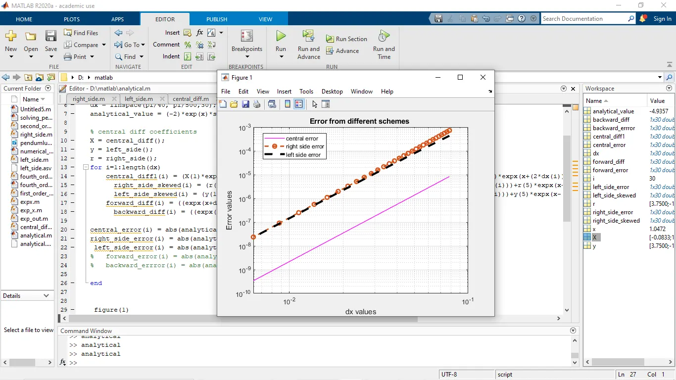
`->` As you can see the above plot has shown the comparison of the central diff, right side Skewed and Skewed left-sided difference for wide range of dx values, if you observe you can see that the central difference scheme has the higher error as compared to other two schemes . If we see the right side Skewed and Skewed left-sided difference's error is very much similar as both the schemes uses the number of data point to obtain the results

`->`So we have been asked that skeweds schemes are more usefull than the central diff. scheme

so let us first see where skewed are used, they are used for calculating the corner points or nodes which have high approximation values and works very good when there are less points are available on one side of grid and for central schemes we need both the points then and then only we can have the correct results and as we know every complete info may not be given to us or not available.