Week 7 - Simulation of a 1D Super-sonic nozzle flow simulation using Macormack Method

AIM

To simulate the isentropic flow through a quasi 1D subsonic-supersonic nozzle.

To determine the steady-state distribution of primitive variables inside the nozzle.

To simulate find Time-wise variation of the primitive variables.

To simuate the variation of Mass flow rate distribution inside the nozzle at different time steps during the time-marching process.

To compare the Normalized mass flow rate distributions of both forms.

DEFINITIONS OF THE TERMS USED

NOZZLE

A nozzle is a device which is used to give the direction to the gases coming out of the combustion chamber. Nozzle is a tube which has the capacity to convert the thermo-chemical energy generated in the combustion chamber into kinetic energy. The nozzle converts the low velocity, high pressure, high temperature gas in the combustion chamber into high velocity gas of lower pressure and low temperature. In a nozzle, the velocity of fluid increases at the expense of its pressure energy.

CONVERGENT DIVERGENT NOZZLE

An arrangement in which the forward portion of the nozzle is convergent, which increases the pressure of the exhaust gases, while the aft section is divergent to increase gas velocity to the supersonic speed and avoid losses from underexpansion.

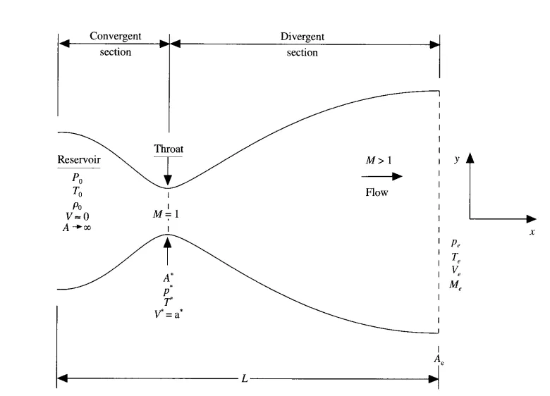
SUBSONIC-SUPERSONIC NOZZLE

Convergent-divergent type of nozzles are mostly used for supersonic flows because it is impossible to create supersonic flows (mach number more than one) in convergent type of nozzle and therefore it restricts us to a limited amount of mass flow through a particular nozzle. In convergent-divergent type of nozzles we can increase the flow velocity much higher than sonic velocity that is why these type of nozzles have a wide applications such as propelling nozzles in jet engines or in air intake for engines working at high rpms.

FLOW FIELD VARIABLES

`T'=T/T_0`

`rho' = rho/rho_0`

`x' = x/L`

`a_0 = sqrt(gammaRT)`

`V' = V/a_0`

`t'=t/(L/a_0)`

`A' = A/Aast`

Where T is temperature, `rho` is density, X is length, V is velocity, `a_0`is velocity of sound, t is time and A is area, all are expressed in dimensionless form and are indicated using superscript`'`.

GOVERNING EQUATIONS

The flow field variables are expressed in non-dimensional form

NON-CONVECTIVE FORM

CONTINUITY - `(delrho')/(delt') = -rho'(delv')/(delx')-rho'V'del((lnA'))/(delx')-V'(delrho')/(delx')`

MOMENTUM - `(delV')/(delt') = -V'(delV')/(delx')-1/gamma((delT)/(delx')+(T')/(rho')(delrho')/(delx'))`

ENERGY - `(delT')/(delt')=-V'(delT')/(delx')-(gamma-1)T'[(delV')/(delx')+V'del((lnA'))/(delx')]`

CONSERVATIVE FORM

CONTINUITY - `del((rho'A'))/(delt')+del((rho'A'V'))/(delx')=0`

MOMENTUM - `del((rho'A'V'))/(delt')+del([rho'A'V'^2+(1/gamma)p'A'])/(delx') = 1/gammap'(delA')/(delx')`

ENERGY - `del([rho'((e')/(gamma-1)+gamma/2V'^2)A'])/(delt')+del([rho'((e')/(gamma-1)+gamma/2V'^2)V'A'+p'A'V'])/(delx')=0`

Simplifying the above equation

`U_1 = rho'A'`

`U_2=rho'A'V'`

`U_3 = rho'((e')/(gamma-1)+gamma/2V'^2)A'`

`F_1 = rho'A'V'`

`F_2 = rho'A'V'+1/gammap'A'`

F_3 = `rho'((e')/(gamma-1)+gamma/2V'^2)V'A'+p'A'V'`

`J_2 = 1/gammap'(delA')/(delx')`

Where `U_1,U_2,U_3` are the solution vectors and `F_1,F_2,F_3` are the flux vectors.

FORMULAS USED

MACCORMACK METHOD

The MacCormack method is an explicit finite difference technique which is a second order accurate in both space and time.

PREDICTOR STEP

The initial, "prediction" step, starts from a function fitted to the function-values and derivative-values at a preceding set of points to extrapolate ("anticipate") this function's value at a subsequent, new point.

Predictor step uses forward differencing for the space terms.

To get the final solution update `f_i=f_i+(delf)/(delt_p)Deltat`is used which is derived from Taylor series.

CORRECTOR STEP

Corrector step refines the initial approximation by using the predicted value of the function and another method to interpolate that unknown function's value at the same subsequent point.

It uses backward differencing for the space terms.

`(delf)/(delt_(avg)) = 0.5((delf)/(delt_p)+(delf)/(delt_c))` where `(delf)/(delt_p)`is the predictor time function and `(delf)/(delt_c)`is the corrector time function, which are derived using the space functions accordingly.

To get the final solution update `f_i=f_i+(delf)/(delt_(avg))Deltat`is used.

TIME STEP

`Deltat_i = C.(Deltax)/(a_i+v_i)`

where `a_i`is speed of sound

C is Courant number(CFL = 0.5)

`v_i`velocity

BASIC FORMULAS USED

Area = `1+2.2.(x-1.5)^2` `0lexle3`

Pressure = `rho.T`

Mass flow rate = `rho.A.V`

Mach no = `V/sqrtT`

BOUNDARY CONDITIONS

Boundary for conservative form

Inlet

`u1(1) = a(1);`

`u2(1)=2astu2(2)-u2(3);`

`u3(1)=2astu3(n-1)-u3(n-3);`

outlet conditions

`u1(n) = 2astu(n-1)-u1(n-2);`

`u2(n)=2astu2(n-1)-u2(n-2);`

`u3(n)=2astu3(n-1)-u3(n-2);`

Boundary for non-conservative

Inlet

`v(1)=2astv(2)-v(3);`

Outlet

`v(n)=2astv(n-1)-v(n-2)`

`rho(n)=2astrho(n-1)-rho(n-2)`

`t(n)=2astt(n-1)-t(n-2)`

MAIN PROGRAM

clear all
close all
clc

%inputs
n =31;
x = linspace(0,3,n);
dx =x(2)-x(1); %x(2)-x(1);
nt = 1400;
CFL = 0.5;
gamma = 1.4;
throat = 16;
[pressure,rho,t,v,mach_no,mass_flow_rate,throat_t,throat_pressure,throat_mass_flow_rate,throat_rho,throat_mach_no] = non_conservative(n,x,dx,nt,throat,CFL,gamma)
[con_pressure,con_rho,con_t,con_v,con_mach_no,con_mass_flow_rate,con_throat_mass_flow_rate,con_throat_pressure,con_throat_t,con_throat_rho,con_throat_mach_no] = conservative(n,x,dx,nt,throat,CFL,gamma)
        
        
figure(1)

figure(2)

figure(3)

figure(4)

figure(6)

figure(7)
plot(x,mass_flow_rate)
hold on
plot(x,con_mass_flow_rate)
xlabel('length of the nozzle')
ylabel('mass flow rate')
legend('non-conservative','conservative')
title('comparison of mass flow rate of conservative and non-conservative')

CODE EXPLANATION

The main program consists of the inputs such as number of nodes, length of the nozzle, distance between the grid points common for both forms and it calls the and executes the function and plots using it.

Non-Conservative function code explanation

Firstly, Non-Conservative functions calculates the initial profiles such as area, density, and pressure, etc and the time step using the formuals listed above.

Then, in the next step the time loop is executed, and a copy of the primitive variables is stored for the forthcoming use in finding the final exact values of the primitive variables.

After the previous step, discretization is done using the MacCormack method where the predictor step(the predictor and the corrctor formula is listed above) is executed, the solution is updated, which inturn is used in the corrector step and the solution for corrector step is also executed.

Following this, the arithmetic mean of predictor and corrector solution is executed and these values are used in calculating the final solution using the initial primitive variables.

Furthermore, the boundary values are updated and the mach number, pressure and mass flow rate values are executed using their basic formulas.

Finally, the throat values of all the primitive variables is found by assigning the throat node, which is 16 in this case.

Conservative function code explanation

The code for conservative function is similar to non-conservative, except instead of the primitive values being used solution vectors and flux variables(both list above) is used in the predictor and corrector step and these values are relatively used to find the primitive variables.

Finally, the plots are graphed comparing the variables as per the objective of the program.

Non_conservative function

function[pressure,rho,t,v,mach_no,mass_flow_rate,throat_t,throat_pressure,throat_mass_flow_rate,throat_rho,throat_mach_no] = non_conservative(n,x,dx,nt,throat,CFL,gamma)
% calculating Initial profiles
rho=1-0.3146*x;
t=1-0.2314*x;
v=(0.1+1.09*x).*(t).^0.5;

%area
a=1+2.2*(x-1.5).^2;
air = t.^(1/2);%speed of sound
dt = min((CFL*dx)./(v+air));

%time steps
 %outer time step
 for i=1:nt
    rho_old=rho;
    v_old=v;
    t_old=t;
%     %predictor method
    for j=2:n-1
        dvdx=(v(j+1)-v(j))/dx;
        drhodx=(rho(j+1)-rho(j))/dx;
        dtdx=(t(j+1)-t(j))/dx;
        dlogadx=(log(a(j+1))-log(a(j)))/dx;
        
        %contuinity equation
        drhodt_p(j)=-rho(j)*dvdx-rho(j)*v(j)*dlogadx-v(j)*drhodx;       
        %Momentum equation
        dvdt_p(j)=-v(j)*dvdx-(1/gamma)*(dtdx+(t(j)/rho(j))*drhodx);       
        %energy equation
        dtdt_p(j)=-v(j)*dtdx-(gamma-1)*t(j)*((dvdx+v(j)*dlogadx));
         
    end
    
    for j=2:n-1
      %solution update
      rho(j)=rho(j)+drhodt_p(j)*dt;
      v(j)=v(j)+dvdt_p(j)*dt;
      t(j)=t(j)+dtdt_p(j)*dt;   
    end
    
    %corrector method
    for j=2:n-1
        dvdx = (v(j)-v(j-1))/dx;
        drhodx = (rho(j)-rho(j-1))/dx;
        dtdx = (t(j)-t(j-1))/dx;
        dlogadx = (log(a(j))-log(a(j-1)))/dx;
        
        %contuinity equation
        drhodt_c(j)=-rho(j)*dvdx-rho(j)*v(j)*dlogadx-v(j)*drhodx;     
        %momentum equation
        dvdt_c(j)=-v(j)*dvdx-(1/gamma)*(dtdx+(t(j)/rho(j))*drhodx);      
        %energy equation
        dtdt_c(j)=-v(j)*dtdx-(gamma-1)*t(j)*((dvdx+v(j)*dlogadx));
    end    
        %computing the average time derivative
        drhodt=0.5*(drhodt_p+drhodt_c);
        dvdt=0.5*(dvdt_p+dvdt_c);
        dtdt=0.5*(dtdt_p+dtdt_c);
        
   %final Solution update
    for j=2:n-1
    rho(j)=rho_old(j)+drhodt(j)*dt;
    v(j)=v_old(j)+dvdt(j)*dt;
    t(j)=t_old(j)+dtdt(j)*dt;    
    end
        
        %applying the boundary condition
        %inlet
        v(1)=2*v(2)-v(3);

        %outlet
        v(n)=2*v(n-1)-v(n-2);
        rho(n)=2*rho(n-1)-rho(n-2);
        t(n)=2*t(n-1)-t(n-2);
        
        %calculating pressue, mass flow rate and mach no
        pressure = rho.*t;
        mach_no = v./(t.^(1/2));
        mass_flow_rate = rho.*a.*v;
        
        %assigning primitive variables at throat at node16
        throat_mach_no(i) = mach_no(throat);
        throat_t(i) = t(throat);
        throat_pressure(i) = pressure(throat);
        throat_rho(i) = rho(throat);
        throat_mass_flow_rate(i) = mass_flow_rate(throat);
        
        figure(3)
        if i==1
            plot(x,mass_flow_rate,'y')
            hold on
        elseif i==50
            plot(x,mass_flow_rate,'r')
            hold on
        elseif i==100
            plot(x,mass_flow_rate,'b')
            hold on
        elseif i==150
            plot(x,mass_flow_rate,'g')
            hold on
        elseif i==200
            plot(x,mass_flow_rate,'m')
            hold on
        elseif i ==700
            plot(x,mass_flow_rate,'c')
            hold on
            elseif i ==1400
                plot(x,mass_flow_rate,'k')
                hold on
        end
 end
legend('0dt','50dt','100dt','150dt','200dt','700dt','1400dt')
xlabel('non-dimensional mass flow')
ylabel('non-dimensional distance through nozzle')
title('Non-conservative: Variation of Mass flow rate distribution inside the nozzle at different time steps during the time-marching process')

        
figure(1)
%plotting steady state primitive variables 
subplot(4,1,1)
plot(x,mach_no,'g')
xlabel('length of the nozzle')
ylabel('mach no')
title('steady state distribution of primitive variables(Non-Conservative form)')
subplot(4,1,2) 
plot(x,t,'b')
xlabel('length of the nozzle')
ylabel('temperature rate')
subplot(4,1,3) 
plot(x,rho,'c')
xlabel('length of the nozzle')
ylabel('density rate')
subplot(4,1,4) 
plot(x,pressure,'r')
xlabel('length of the nozzle')
ylabel('pressure rate')

figure(2)
subplot(4,1,1) 
%plotting primitive variables        
plot(throat_mach_no,'g')
xlabel('time iterations')
ylabel('mach no')
title('timewise variations of primitive variables at throat(Non-Conservative form)')
subplot(4,1,2) 
plot(throat_t,'b')
xlabel('time iterations')
ylabel('temperature rate')
subplot(4,1,3) 
plot(throat_rho,'c')
xlabel('time iterations')
ylabel('density rate')
subplot(4,1,4) 
plot(throat_pressure,'r')
xlabel('time iterations')
ylabel('pressure rate')

end

Conservative function

function[con_pressure,con_rho,con_t,con_v,con_mach_no,con_mass_flow_rate,con_throat_mass_flow_rate,con_throat_pressure,con_throat_t,con_throat_rho,con_throat_mach_no] = conservative(n,x,dx,nt,throat,CFL,gamma)
%area
con_a = 1+2.2*((x-1.5).^2);
%initial conditions
for k = 1:n
    if x(k)>=0 && x(k)<=0.5
        con_rho(k)= 1;
        con_t(k)=1;
    elseif x(k)>=0.5 && x(k)<=1.5            
            con_rho(k) = 1-0.366*(x(k)-0.5);            
            con_t(k) = 1-0.167*(x(k)-0.5);
    elseif x(k)>=1.5 && x(k)<=3.5                
                con_rho(k) = 0.634-0.3879*(x(k)-1.5);
                con_t(k) = 0.833-0.3507*(x(k)-1.5);
    end
end
con_v = 0.59./(con_rho.*con_a);
%solution variables initialization
u1 = con_rho.*con_a;
u2 = con_rho.*con_v.*con_a;
u3 = con_rho.*((con_t/(gamma-1)+(gamma/2).*con_v.^2).*con_a);
air = con_t.^(1/2);%speed of sound
dt = min((CFL*dx)./(con_v+air));

%time step
for i = 1:nt
    u1_old  = u1;
    u2_old = u2;
    u3_old = u3;
    
    %flux vectors
    f1 = u2;
    f2 = (u2.^2./u1)+((gamma-1)/gamma)*(u3-(gamma/2).*(u2.^2)./u1);
    f3 = (gamma.*u2.*u3)./u1-(gamma*((gamma-1)/2)*(u2.^3)./u1.^2);    
        
    %predictor step
    for j=2:n-1
        %space term
      %  j2(j)=(1/gamma)*(rho(j)*t(j))*((a(j)-a(j-1))/dx);  Forward differencing to be used
        j2(j)=(1/gamma)*(con_rho(j)*con_t(j))*((con_a(j+1)-con_a(j))/dx);
        %continuity equation
        du1dt_p(j) = -(f1(j+1)-f1(j))/dx;
        %momentum equation
        du2dt_p(j) = -(f2(j+1)-f2(j))/dx+j2(j);
        %energy equation
        du3dt_p(j) = -(f3(j+1)-f3(j))/dx;
        
        %solution update
        u1(j) = u1(j)+du1dt_p(j)*dt;
        u2(j) = u2(j)+du2dt_p(j)*dt;
        u3(j) = u3(j)+du3dt_p(j)*dt;
    end
        
        %updating primitive variables
        con_rho = u1./con_a;
        con_t = (gamma-1).*((u3./u1)-(gamma/2).*(u2./u1).^2);
        con_v = u2./u1;        
        
        %updating flux vectors
         f1 = u2;
         f2 = (u2.^2./u1)+((gamma-1)/gamma)*(u3-(gamma*u2.^2)./(2*u1));
         f3 = (gamma*u2.*u3)./u1-gamma*((gamma-1)/2)*(u2.^3./u1.^2);    
        
         %corrector method
         for j = 2:n-1
         j2(j)=(1/gamma)*(con_rho(j)*con_t(j))*((con_a(j)-con_a(j-1))/dx);  %Backward differencing
         %continuity equation
         du1dt_c(j) = -(f1(j)-f1(j-1))/dx;
         %momentum equation
         du2dt_c(j) = -(f2(j)-f2(j-1))/dx+j2(j);
         %energy equation
         du3dt_c(j) = -(f3(j)-f3(j-1))/dx;
         end
         
         %finding average time derivative
         du1dt_a = 0.5.*(du1dt_p+du1dt_c);
         du2dt_a = 0.5.*(du2dt_p+du2dt_c);
         du3dt_a = 0.5.*(du3dt_p+du3dt_c);
         
         %final solution update
         for j = 2:n-1
             u1(j) = u1_old(j)+du1dt_a(j)*dt;
             u2(j) = u2_old(j)+du2dt_a(j)*dt;
             u3(j) = u3_old(j)+du3dt_a(j)*dt;
         end
             
             %final update of premitive variables
             con_rho = u1./con_a;
             con_t = (gamma-1).*((u3./u1)-(gamma/2).*(u2./u1).^2);
             con_v = u2./u1;
             
             %boundary conditions
             %inlet
             u1(1)=con_a(1);
             u2(1)=2*u2(2)-u2(3);
             u3(1)=u1(1)*(con_t(1)/(gamma-1)+(gamma/2)*(con_v(1))^2);
             
             %outlet
             u1(n)=2*u1(n-1)-u1(n-2);
             u2(n)=2*u2(n-1)-u2(n-2);
             u3(n)=2*u3(n-1)-u3(n-2);
             
             %calculating pressure, mass flow rate,mach no
             con_pressure = con_rho.*con_t;
             con_mach_no = con_v./(con_t.^(1/2));
             con_mass_flow_rate = con_rho.*con_a.*con_v;
             
             %calculating pressure, mass flow rate,mach no at throat
             con_throat_mach_no(i) = con_mach_no(throat);
             con_throat_t(i) = con_t(throat);
             con_throat_pressure(i) = con_pressure(throat);
             con_throat_rho(i) = con_rho(throat);
             con_throat_mass_flow_rate(i) = con_mass_flow_rate(throat);
             
        figure(6)
        if i==1
            plot(x,con_mass_flow_rate,'y')
            hold on
        elseif i==50
            plot(x,con_mass_flow_rate,'r')
            hold on
        elseif i==100
            plot(x,con_mass_flow_rate,'b')
            hold on
        elseif i==150
            plot(x,con_mass_flow_rate,'g')
            hold on
        elseif i==200
            plot(x,con_mass_flow_rate,'m')
            hold on
        elseif i ==700
            plot(x,con_mass_flow_rate,'c')
            hold on
            elseif i ==1400
                plot(x,con_mass_flow_rate,'k')
                hold on
        end
end
        legend('0dt','50dt','100dt','150dt','200dt','700dt','1400dt')
        xlabel('non-dimensional mass flow')
        ylabel('non-dimensional distance through nozzle')
        title('conservative: Variation of Mass flow rate distribution inside the nozzle at different time steps during the time-marching process')
         figure(4)
        %plotting steady state primitive variables 
        subplot(4,1,1)       
        plot(x,con_mach_no,'g')
        xlabel('length of the nozzle')
        ylabel('mach no')
        title('steady state distribution of primitive variables(Conservative form)')
        subplot(4,1,2) 
        plot(x,con_t,'b')
        xlabel('length of the nozzle')
        ylabel('temperature rate')
        subplot(4,1,3) 
        plot(x,con_rho,'c')
        xlabel('length of the nozzle')
        ylabel('density rate')
        subplot(4,1,4) 
        plot(x,con_pressure,'r')
        xlabel('length of the nozzle')
        ylabel('pressure rate')
        
        figure(5)
        subplot(4,1,1) 
        %plotting primitive variables        
        plot(con_throat_mach_no,'g')
        xlabel('time iterations')
        ylabel('mach no')
        title('timewise variations of primitive variables at throat(Conservative form)')
        subplot(4,1,2) 
        plot(con_throat_t,'b')
        xlabel('time iterations')
        ylabel('temperature rate')
        subplot(4,1,3) 
        plot(con_throat_rho,'c')
        xlabel('time iterations')
        ylabel('density rate')
        subplot(4,1,4) 
        plot(con_throat_pressure,'r')
        xlabel('time iterations')
        ylabel('pressure rate')
end

FIGURE 1

NON-CONSERVATIVE: STEADY STATE DISTRIBUTION OF PRIMITIVE VARIABLES

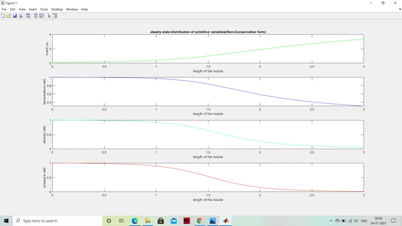
FIGURE 2

NON-CONSERVATIVE: TIMEWISE VARIATIONS OF PRIMITIVE VARIABLES AT THROAT

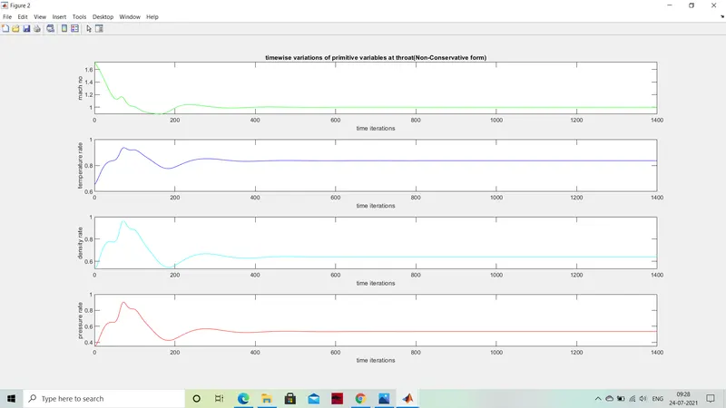
FIGURE 3

NON-CONSERVATIVE: VARIATIONS OF MASS FLOW RATE AT DIFFERENT TIME STEPS DURING THE TIME MARCHING PROCESS

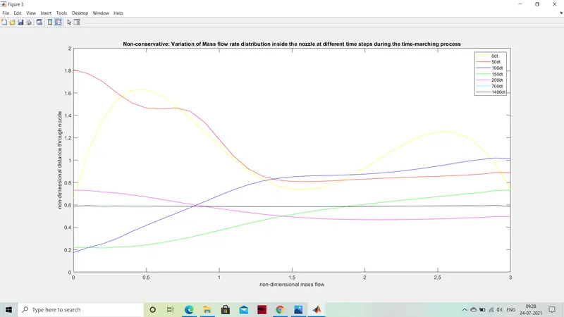
FIGURE 4

CONSERVATIVE: STEADY STATE DISTRIBUTION OF PRIMITIVE VARIABLES

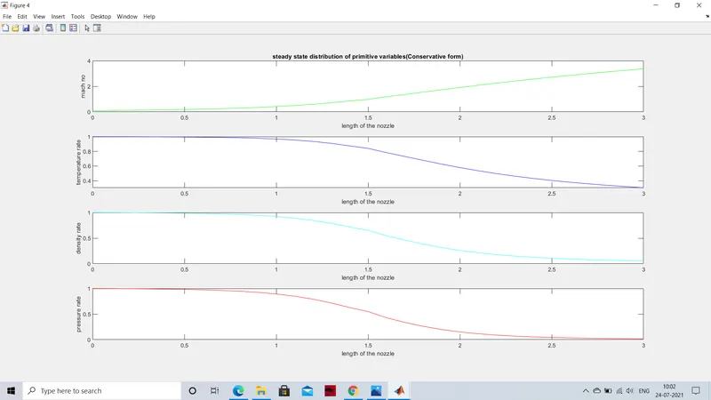
FIGURE 5

CONSERVATIVE: TIMEWISE VARIATIONS OF PRIMITIVE VARIABLES AT THROAT

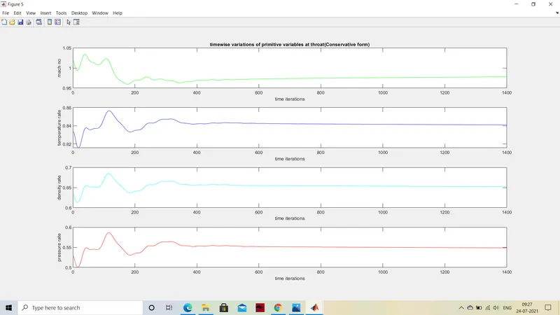
FIGURE 6

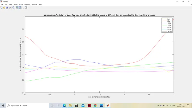
CONSERVATIVE: VARIATIONS OF MASS FLOW RATE AT DIFFERENT TIME STEPS DURING THE TIME MARCHING PROCESS

OBSERVATION

As seen in figure 1 and 4, all the primitive values such as density, temperature, pressure decreases along the length of the nozzle, but the mach no increases.

In figure 2 and 5, the primitive variables at different time steps shows there was some fluctuations in the initial steps and became steady which indicates the solution has reached steady state.

It can be observed from figure 3 and 6, there was no change in the mass flow rate after 700 iterations iteslf and the additional time steps until 1400 iterations remained same indicating the steady state achievement.

FIGURE 7

COMPARISON OF MASS FLOW RATE OF CONSERVATIVE AND NON-CONSERVATIVE

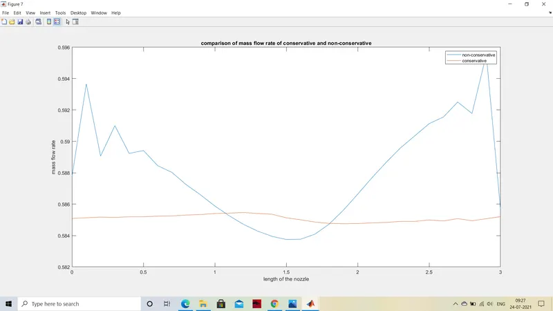
From figure 7, it can be seen that mass flow rate in more stable in conservative form as compared to the non-conservative form.

GRID INDEPENDENCE

By changing the number of nodes to 61 and the throat node we got sligtly better results.

The same is true for all locations within the nozzle. In short, the two steady state numerical solutions are essentilly the same, and therefore it can be concluded that the original calculations using 31 grid points is essentially grid-independent.

DEMONSTATION OF GRID INDEPENDENCE AT THE THROAT

	FORMS	`rho^ast/rho_0`	`T^ast/T_0`	`p^ast/p_0`	`M`
CASE 1 :31 NODES	CONSERVATIVE FORM NON-CONSERVATIVE	0.6525 0.6387	0.8413 0.8365	0.5487 0.5342	0.9780 0.9994
CASE 2: 61 NODES	CONSERVATIVE FORM NON-CONSERVATIVE	0.5929 0.5940	0.8109 0.8121	0.4807 0.4824	1.0858 1.0826
EXACT ANALYTICAL SOLUTIONS	-	0.634	0.833	0.528	1.000

From the above test we can can see that conservation form is time consuming but it's more stable than the non_conservative form.

The conservative form solutions are closer to the exact the solution.

CONCLUSION

The Non-Conservative is faster, easier and converges fast as the primitive variables are used directly.

While the conservation form produces more stable results as it uses flux variables.