Week 7 - Auto ignition using Cantera

AIM

• To simulate the Auto Ignition Time for Methane under the following conditions

1. Methane with a constant temperature of 1250K and pressure varying from 1 to 5 atm.
2. Methane with a constant pressure of 5 atm and temperature varying from 950K to 1450K

• To find the rate of change of molar concentrations of the given elements "H2O, O2, OH" with respect to the time.

1. When Temperature is 1000K and pressure 5 bar
2. When Temperature is 500K and pressure 5 bar

Introduction:

Auto ignition

Auto ignition occurs when a mixture of gases or vapors ignites spontaneously with no external ignition source and after reaching a certain temperature, the autoignition temperature. The autoignition temperature is not an intrinsic property of the gases or vapors but is the lowest temperature in a system where the rate of heat evolved from the gases or vapors increases beyond the rate of heat loss to the surroundings, resulting in ignition. The autoignition temperature of a mixture of gases or vapors is affected by pressure, vessel shape and volume, surface activity, contaminants, flow rate, reaction rate, droplet and mist formation, gravity, and reactant concentration.

Theory:

Ignition delay

Ignition delay time (IDT) is the time needed for a mixture of fuel and oxidizer to react at a certain temperature and pressure. This delay time is an important parameter for the engine designer and is typically determined experimentally. An experimental device capable of producing high-temperature and high-pressure conditions to perform such measurements is the shock tube.

It's found when the initial temperature raeaches 400k

Ignition delay = initial temperaure + 400k

Applications:

Controlled Auto-Ignition combustion, also known as Homogeneous Charge Compression Ignition, has the potential to simultaneously reduce the fuel consumption and nitrogen oxides emissions of gasoline engines.

Code explanation

Initially I imported the required modules and created a gas object and provided the initial values

Secondly I created the rector using the IdealGasReactor command followed by ReactorNet command

Foolowing it I made use of the advance command to run the reactor at the new instance

Instead of using specifyng different attributes individully I made use of the state object and got the required temperature and pressure using it.

CASE 1:

PART1: Methane with a constant temperature of 1250K and pressure varying from 1 to 5 atm.

import matplotlib.pyplot as plt
import cantera as ct
import numpy as np

gas = ct.Solution('gri30.xml')
T= 1250

pressure = np.linspace(1*ct.one_atm,5*ct.one_atm,5)
ignition_delay = []

for P in pressure:
	gas.TPX = T,P,{'CH4':1,'O2':2,'N2':7.52}
	r = ct.IdealGasReactor(gas)
	sim=ct.ReactorNet([r])
	T_old= T
	time = 0

	states = ct.SolutionArray(gas,extra=['t_ms','t'])

	for i in range(1000):
		time+= 1e-3
		sim.advance(time)
		states.append(r.thermo.state,t_ms = time*1e3,t = time)
		T_new = states.T
		T_new = T_new[i-1]

		if (T_new>=400+T_old):
			ignition_delay.append(time)
		T_old = states.T
		T_old = T_old[i-1]

		plt.figure(1)
		plt.plot(states.t_ms,states.T)
		plt.xlabel('time')
		plt.ylabel('temperature')
		plt.legend(['1bar','2bar','3bar','4bar','5bar'])

plt.figure(2)
plt.plot(pressure,ignition_delay)
plt.xlabel('pressure')
plt.ylabel('igntion delay')
plt.show()

Plot

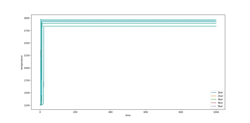
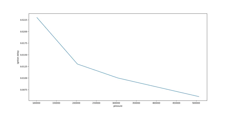
PART2:Methane with a constant pressure of 5 atm and temperature varying from 950K to 1450K

import matplotlib.pyplot as plt
import cantera as ct
import numpy as np

gas = ct.Solution('gri30.xml')
P=5*101325

temperature = np.linspace(950,1450,5)
ignition_delay = []

for T in temperature:
	gas.TPX = T,P,{'CH4':1,'O2':2,'N2':7.52}
	r = ct.IdealGasReactor(gas)
	sim=ct.ReactorNet([r])
	T_old= T
	time = 0

	states = ct.SolutionArray(gas,extra=['t_ms','t'])

	for i in range(1000):
		time+= 1e-3
		sim.advance(time)
		states.append(r.thermo.state,t_ms = time*1e3,t = time)
		T_new = states.T
		T_new = T_new[i-1]

		if (T_new>=400+T_old):
			ignition_delay.append(time)
		T_old = states.T
		T_old = T_old[i-1]

		plt.figure(1)
		plt.plot(states.t_ms,states.T)
		plt.xlabel('time')
		plt.ylabel('temperature')
		plt.legend(['950','1075','1200','1325','1450'])

plt.figure(2)
plt.plot(temperature,ignition_delay)
plt.xlabel('temperature')
plt.ylabel('igntion delay')
plt.show()

plot

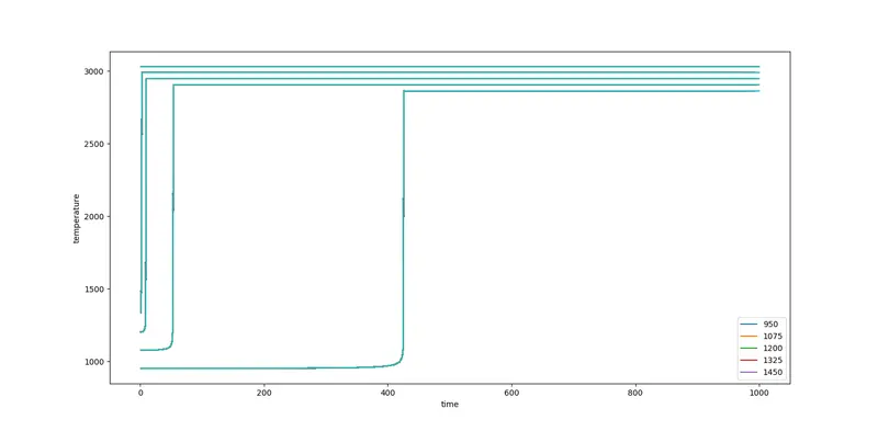
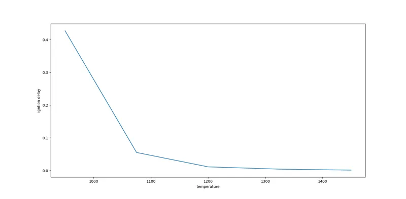
The rate of change of molar concentrations of the given elements "H2O, O2, OH" with respect to the time when Temperature is 1000K and 500k and pressure 5 bar

import matplotlib.pyplot as plt
import cantera as ct
import numpy as np

gas = ct.Solution('gri30.xml')
temperature = [500,1000]
P = 5*101325

for T in temperature:
	gas.TPX = T,P,{'CH4':1,'O2':2,'N2':7.52}
	r = ct.IdealGasReactor(gas)
	sim = ct.ReactorNet([r])
	time = 0

	states = ct.SolutionArray(gas,extra = ['time_in_ms','t'])
	for i in range(10000):
		time += 1e-3
		sim.advance(time)
		states.append(r.thermo.state,time_in_ms = time*1e3,t= time)

	plt.figure()

	plt.subplot(3,1,1)
	plt.plot(states.t,states.X[:,gas.species_index('O2')])
	plt.xlabel('Time')
	plt.ylabel('X_O2')
	plt.title('Mole fractions at 500k and 1000k and 5bar')

	plt.subplot(3,1,2)
	plt.plot(states.t,states.X[:,gas.species_index('H2O')])
	plt.xlabel('Time')
	plt.ylabel('X_H2O')

	plt.subplot(3,1,3)
	plt.plot(states.t,states.X[:,gas.species_index('OH')])
	plt.xlabel('Time')
	plt.ylabel('X_OH')
	plt.show()

PLOT

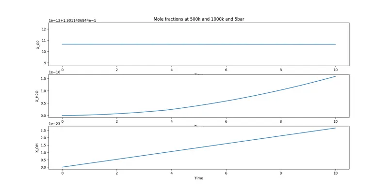
At temperaure 500k and pressure 5bar

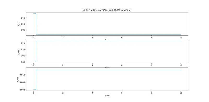
At temperaure 1000k and pressure 5bar

Conclusion

As initial temperature or pressure values are increased ignition delay reaches zero and stays constant.

Ignition delay is highly affected by varying temperature than varying pressure

Molar concentration of O2 remains constant at 500k and 5bar whereas H2O and OH followed a similar pattern. Concentration of O2 decreases at 1000k and 5bar and vice versa for OH, H2O.