Simulation of a 1D Super-sonic nozzle flow simulation using Macormack Method in MATLAB
Simulate the isentropic flow through a quasi 1D subsonic-supersonic nozzle using both the conservation and non-conservation forms of the governing equations.
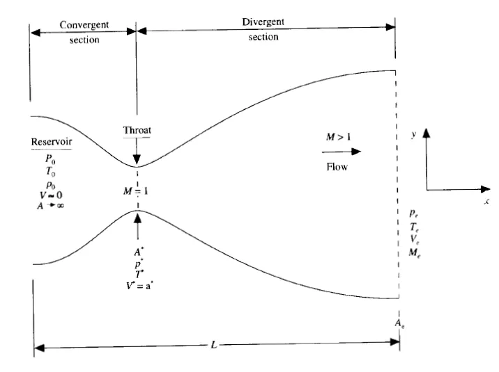
Problem description : The geometry under consideration is a steady state isentropic flow in a convwrgent-divergent nozzle. The flow at the inlet comes from a reservoir where the temperature and pressure are denoted as `T_0` and `p_o` respectively. The reservoir is considered to be very large, and hence as the area tends towards infinity, the inlet velocity tends towards zero. The flow expands isentropically to supersonic speeds at the nozzleexit, where the exit velocity, temperature , pressure and mach number are denoted as `v_e`, `T_e` , `p_e` and `M_e` respectively. The flow is locally subsonic in the convergent section sonic at the throat area and supersonic in the divergent section. At the throat area since the speed is sonic, the local velocity of the flow is equal to the speed of sound. Eventhough the cross-sectional area of the nozzle varies, an assumption is made that the fow properties vary only in the x-direction, hence the flow is said to be a quasi-1D flow.
Diagramatic representation of the geometry :
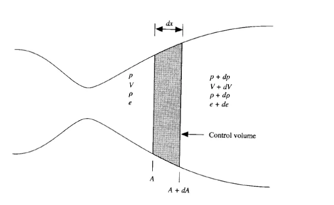
For the derivations, a control volume is selected. The control volume is denoted as the shaded region in the below image.
Governing equations :
1. Continuity Equation :
Lets consider the integral form of the continuity equation
`del/(delt)intintintrhodelV + intintrhoVdS = 0`
Applying this to the shaded region we get,
`del/(delt)intintintrhodelV = del/(delt)(rhoAdx)`
Where `Adx` is the volume of the control volume.
`intintrhoVdS = -rhoVA + (rho+drho)(V + dV)(A + dA) = d(rhoAV)`
Hence ,
`del/(delt)(rhoAdx) + d(rhoAV) = 0`
dividing by dx , we get
`del/(delt)(rhoA) + del/(delx)(rhoAV) = 0`
This is the conservative form of the continuity equation.
Expanding this equation we get ,
`del/(delt)(rhoA) + rhoA(delV)/(delx) + rhoV(delA)/(delx) + VA(delrho)/(delx) = 0`
This is the non-conservative form of the continuity equation.
2. Momentum Equation
The integral form of the x-component of the momentum equation is :
`del/(delt) int int int rhoudV + int int (rhouV)dS = - int int (pdS)_x`
Applying this equation to the control volume, we get
`del/(delt)int int int rhoudV = del/(delt)(rhoVAdx)`
`int int (rhouV)dS = -rhoV^2A + (rho +drho)(V+dV)^2(A+dA)`
`int int pdS = -pA + (p +dp)(A+dA) - pdA`
Substituting these equations , we get
`del/(delt)(rhoVAdx) - rhoV^2A + (rho+drho)(V+dV)^2(A+dA) = pA - (p +dp)(A +dA) + pdA`
Simplifying and neglecting higher order terms, we get
`del/(delt)(rhoVAdx) + d(rhoV^2A) = -Adp`
dividing by `dx`
`del/(delt)(rhoVA) + del/(delx)(rhoV^2A) = -A(delp)/(delx)`
This is the conservative form of the momentum equation. Obtaining the equivalent non-conservative form, this can be done by multiplying the continuity equation by `V`
`Vdel/(delt)(rhoA) + V(del(rhoVA))/(delx) = 0`
Subtraction this from the conservative form of the momentum equation
`del/(delt)(rhoVA) - Vdel/(delt)(rhoA) + del/(delx)(rhoV^2A) - V del/(delx)(rhoV^2A) = -A(delp)/(delx)`
Simplifying, we get the non-conservative form of the momentum equation
`rho(delV)/(delt) + rhoV(delV)/(delx) = -(delp)/(delx)`
3. Energy Equation
Consider the integral form of the energy equation
`del/(delt)int intint rho(e + (V^2/2))dV + int int rho(e + (V^2/2))V.dS = - int int (pV)dS`
Applying to the control volume, we get
`del/(delt)[rho(e+(V^2/2))Adx] - rho(e+(V^2/2))VA + (rho+drho)[(e+de) + (V+dV)^2/2](V+dV)(A+dA) =`
`- [-pVA + (p+dp)(V+dV)(A+dA) - 2(pV(dA)/2)]`
Simplifying and neglecting the higher order terms, we get
`del/(delt)[rho(e+V^2/2)Adx] + d(rhoeVA) + d(rhoV^3A/2) = -d(pAV)`
Dividing by `dx`
`del/(delt)[rho(e+V^2/2)A] + del/(delx)[rho(e+V^2/2)VA] = -del/(delx)(pAV)`
From the derivation of the conservative form of the momentum the following equation is consider and multiplied with `V`.
`del/(delt)(rhoV^2A) + del/(delx)(rhoV^3A) = -AV(delp)/(delx)`
subtracting this equation from the conservative form of the energy equation ,
`del/(delt)(rhoeA) + del/(delx)(rhoeVA) = -p*del/(delx)(AV)`
This above equation is the conservative form of the energy equation.
The non-conservative form can be obtained by multiplying `e` with the continuity equation,
`e*(del(rhoA))/(delt) + e* (del(rhoAV))/(delx) = 0`
subtracting this equation from the conservative form of energy equation,
`rhoA(dele)/(delt) + rhoAV(dele)/(delx) = -p(del(AV))/(delx)`
expanding the right hand side and dividing
`rho(dele)/(delt) + rhoV(dele)/(delx) = -p(delV)/(delx) - pV/A(delA)/(delx)`
Simplifying ,
`rho(dele)/(delt) + rhoV(dele)/(delx) = -p(delV)/(delx) - pV(del(ln A))/(delx)`
This is the non-conservative form of the energy equation in terms of internal energy. Considering a calorifically perfect gas, the following equation can be substituted to modify the energy equation in terms of the temperature.
`e = c_vT`
Subtituting this, the energy equation becomes,
`rhoc_v(delT)/(delt) + rhoVc_v(delT)/(delx) = -p(delV)/(delx) - pV(del(ln A))/(delx)`
All the equation above , there are four unknown variables, but the pressure term can be written in terms of density and pressure.
`p = rhoRT`.
Substituting the above equation, the non-conservative form of the equations for the given case is as follows :
Continuity equation : `(del(rhoA))/(delt) + V(del(rhoA))/(delx) = -rhoA(delV)/(delx)`
Momentum equation : `rho(delV)/(delt) + rhoV(delV)/(delx) = -(delp)/(delx)`
Energy equation : `rho(dele)/(delt) + rhoV(dele)/(delx) = -p(delV)/(delx) - pV(del(ln A))/(delx)`
On the other hand, the conservative form of the equations for the given case is as follows :
Continuity equation : `del/(delt)(rhoA) + del/(delx)(rhoAV) = 0`
Momentum equation : `del/(delt)(rhoVA) + del/(delx)(rhoV^2A) = -A(delp)/(delx)`
Energy equation : `del/(delt)[rho(e+V^2/2)A] + del/(delx)[rho(e+V^2/2)VA] = -del/(delx)(pAV)`
The equations are non-dimensionalised as most of the results are expressed in these non-dimensionalised forms. The non-dimensionalised parameters are as follows :
- The dimensionless area can be defined as the ratio of the local area`(A)` to that of the throat area `(A^**)` . `A^' = A/A^**`
- The dimensionless velocity can be defined as the ratio of the velocity at a point `(V)` to that of the speed of sound (a_0)`. `V^' = V/a_0`.
- The dimensionless length can be defined as the ratio of the distance along the axis `(x)` to that of the total length of the nozzle `(L)`. `x^' = x/L`.
- The dimensionless time can be expressed as `t^' = t/((L/a_0))`.
- The non-dimensional temperature and density are expressed as `T^' = T/T_0` and `rho^' = rho/ rho_0` where `T_0` and `rho_0` are the temperature and pressure of the reservoir respectively.
The non-conservative form of governing equations can be non-dimensionalised. The resulting equations are as follows :
Continuity equation : `(delrho^')/(delt^') = -rho^'(delV^')/(delx^') - rho^'V^'(del(ln A^'))/(delx^') - V^'(delrho^')/(delx^')`
Momentum equation : `(delV^')/(delt^') = V^'(delV^')/(delx^') - 1/gamma[(delT^')/(delx^') + T^'/rho^'(delrho^')/(delx^')]`
Energy equation : `(delT^')/(delt^') = -V^'(delT^')/(delx^') - (gamma-1)T^'[(delV^')/(delx^') + V^'(del(ln A^'))/(delx^')]`.
Similarly ,
The conservative form of governing equations can be non-dimensionalised. The resulting equations are as follows :
Continuity equation :`del/(delt')(rho'A') + del/(delx')(rho'A'V') = 0`
Momentum Equation : `del/(delt')(rho'V'A') + del/(delx')[(rho'V'^2A')+(1/gamma)p'A'] = (1/gamma)*p'(delA')/(delx')`
`del/(delt')[rho'((e')/(gamma-1)+(gamma*V'^2/2))A'] + del/(delx')[rho'((e')/(gamma-1)+(gamma)*V'^2/2)V'A' + p'A'V'] = 0`
The conservative equations for the quasi-one-dimensional flow is expressed in a generic form. They can be expressed as :
`U_1 = rho'A'`
`U_2 = rho'A'V'`
`U_3 = rho'*((e')/(gamma-1) + gammaV'^2/2)A'`
`F_1 = rho'A'V'`
`F_2 = rho'A'V'^2 + 1/gammap'A'`
`F_3 = rho'((e')/(gamma-1) + 1/gammaV'^2)V'A' + p'A'V'`
`J_2 = 1/gammap'(delA')/(delx')`
With these substitution, the equations can be re-written as :
`(delU_1)/(delt') = - (delF_1)/(delx')`
`(delU_2)/(delt') = - (delF_2)/(delx') + J_2`
`(delU_3)/(delt') = - (delF_3)/(delx')`
MacCormack's method of discretization
The macCormack technique is variation from the lax-wendroff method, where in the second order derivative is not calculated, but instead a two step process is followed called as the predictor step and the corrector step.
Firstly, the initial conditions are used to compute the predictor step. In the predictor step, the forward differencing scheme is used to compute the space terms numerically.Lets consider for example a variable, say `h`. In the predictor step, using the initial conditions `((delh)/(delt))_p` can be computed.
Then the solution update is performed, during which the variable value is updated using the initial conditions and the first order derivative term based on the taylor's series expansion. Let consider the updated variable to be `h^**`.
`h^** = h_(i n itial) + ((delh)/(delx))_p*Deltat`.
Secondly, the update values are used to compute the first order derivative. In the corrector step, the backward differencing scheme is used to compute the space terms numerically. This gives the another results for the first order derivative. In this way the `((delh)/(delt))_c` is computed using `h^**` instead of `h_(i nitial)`.
The average of the first order derivative from the predictor steps and the corrected step are used. This method yields a second order accuracy with rather simpler mathematics.
`((delh)/(delt))_(avg) = 1/2*[((delh)/(delt))_p + ((delh)/(delt))_c]`.
Finally, the average value is used to compute the variable at the next time step :
`h^2 = h_(i nitial)^1 + ((delh)/(delt))_(avg)*Deltat`
Calculating the time step :
According to the stability criteria ( Courant-Friedrichs-Lewy condition),
`C = c * (Deltat)/(Deltax) . <= 1`
Where C is the courant number , c is the flow velocity , dt is the timestep and dx is the grid size. Applying this to the above equation :
`Delta t = C* (Deltax)/(a+V)`
Where V is the local flow velocity and a is the local speed of sound. In this case `C<= 1`, in other words, `Deltat` must be less than , or atleast equal to the time it takes for the sound wave to move from one grid to another. The value of `Deltax` is constant throughtout the flow, but the value of a and V are variable. Hence at a given grid point at a given time step , the condition can be written as :
`Deltat_i^t = (C * Deltax)/(a_i^t + V_i^t)`
While for the adjacent grid point :
`Deltat_(i+1)^t = (C * Deltax)/(a_(i+1)^t + V_(i+1)^t)`
In this case either the local time step for each grid point can be calculated and can be used. This method has a faster convergence rate but whether the steady state solution is accurate enough is not certain. Hence rather than utilising the local time stepping method , there is an alternative method wherein the time step is calculated for each grid point and the minimum value is selected. In this manner hte flow field variables at all grid points correspond to the same physical time. In this case the time step is therefore calculated as :
`Deltat = min ( Deltat_1^t , Deltat_2^t, ...... Deltat_N^t)`.
Main Program :
clear all
close all
clc

%% NON-CONSERVATIVE FORM

% inputs
n =31;
x = linspace(0,3,n);
dx = x(2)-x(1);

%function
[mach_nc, velocity_nc, density_nc, temperature_nc,mass_flow_nc,k,v2_nc,T2_nc,rho2_nc,mach2_nc] = non_conserv(n);

% plotting of steady state values of the flow variables
figure(1)

subplot(4,1,1)
plot(x,velocity_nc,'linewidth',1.5);
xlabel('nozzle length');
ylabel('velocity ratio');
title ('NON CONSERVATION FORM');
%subtitle(sprintf('number of iterations = %d',k));
subtitle('steady state distribution of the flow variable along the nozzle length');

subplot(4,1,2)
plot(x,density_nc,'linewidth',1.5);
xlabel('nozzle length');
ylabel('density ratio');

subplot(4,1,3)
plot(x,temperature_nc,'linewidth',1.5);
xlabel('nozzle length');
ylabel('temperature ratio');

subplot(4,1,4)
plot(x,mach_nc,'linewidth',1.5);
xlabel('nozzle length');
ylabel('Mach number');


%% CONSERVATIVE FORM

% inputs
n =31;
x = linspace(0,3,n);
dx = x(2)-x(1);

%function
[mach_c,velocity_c,density_c,temperature_c,mass_flow_c,k,v1_c,T1_c,rho1_c,mach1_c]= conserv(n);

% plotting of steady state values of the flow variables
figure(2)

subplot(4,1,1)
plot(x,velocity_c,'linewidth',1.5);
xlabel('nozzle length');
ylabel('velocity ratio');
title ('CONSERVATION FORM');
%subtitle(sprintf('number of iterations = %d',k));
subtitle('steady state distribution of the flow variable along the nozzle length');

subplot(4,1,2)
plot(x,density_c,'linewidth',1.5);
xlabel('nozzle length');
ylabel('density ratio');

subplot(4,1,3)
plot(x,temperature_c,'linewidth',1.5);
xlabel('nozzle length');
ylabel('temperature ratio');

subplot(4,1,4)
plot(x,mach_c,'linewidth',1.5);
xlabel('nozzle length');
ylabel('Mach number');


figure(3)
plot(x,mass_flow_c,'linewidth',1.5);
hold on
plot(x,mass_flow_nc,'linewidth',1.5);
xlabel (' nozzle length');
ylabel (' mass flow rate ');
legend ('conservative form','non-conservative form');
axis([0,3,0.575,0.6]);
title('Comparison of Normalized mass flow rate distributions');


% plotting the parameters with respect to time for both conservative form and
% non-conservative form
figure(4)

subplot(4,2,1)
plot(v1_c);
axis([0,2000,0.5,1]);
xlabel('time steps');
ylabel('velocity ratio');
title('CONSERVATIVE FORM');

subplot(4,2,3)
plot(T1_c);
axis([0,2000,0.6,1]);
xlabel('time steps');
ylabel('temperature ratio');

subplot(4,2,5)
plot(rho1_c);
axis([0,2000,0.6,1]);
xlabel('time steps');
ylabel('density ratio');

subplot(4,2,7)
plot(mach1_c);
axis([0,2000,0.8,1.3]);
xlabel('time steps');
ylabel('mach number');

subplot(4,2,2)
plot(v2_nc);
axis([0,2000,0.5,1.5]);
xlabel('time steps');
ylabel('velocity ratio');
title('NON-CONSERVATIVE FORM');

subplot(4,2,4)
plot(T2_nc);
axis([0,2000,0.6,1]);
xlabel('time steps');
ylabel('temperature ratio');

subplot(4,2,6)
plot(rho2_nc);
axis([0,2000,0.3,1]);
xlabel('time steps');
ylabel('density ratio');

subplot(4,2,8)
plot(mach2_nc);
axis([0,2000,0.8,1.8]);
xlabel('time steps');
ylabel('mach number');

sgtitle('Time-wise variation of the flow variables');
Non-conservative form
Initial and boundary conditions :
The initial conditions at time t =0 is given as follows :
`rho = 1-0.3146*x`
`T= 1-0.2314*x`
`V = (0.1 + 1.09*x)*sqrt(T)`
`A = 1 + 2.2*(x-1.5)^2`
Subsonic inflow boundary conditions :
`V_1 = 2*V_2 - V_3`
`rho_1 = 1`
`T_1 = 1`
Subsonic outflow boundary conditions :
`V_N = 2*V_(N-1) - V_(N-2)`
`rho_N = 2*rho_(N-1) - rho_(N-2)`
`T_N = 2*T_(N-1) - T_(N-2)`
The matlab function for the non-conservative form of the equation is as follows :
non_conserv.m
function [mach_nc, velocity_nc,density_nc,temperature_nc,mass_flow_nc,k,v2_nc,T2_nc,rho2_nc,mach2_nc] = non_conserv(n)

% inputs
n=31;
x = linspace(0,3,n);
dx = x(2)-x(1);


%calculate initial profile
rho = 1-(0.3146*x) ;   % density
T = 1- (0.2314*x);    % temperture
v = (0.1 + (1.09*x)).*T.^0.5; % velocity
A = 1 + 2.2*(x-1.5).^2;   % area
gamma = 1.4;

% Time steps
nt = 2000;
C = 0.5;

for o = 1:n
    ts(o) = (C*dx/(T(o)^0.5 + v(o)));
end

dt = min(ts);

% outer time loop
for k =1:nt

    % initial values of the flow varaibles
    rho_old = rho;
    T_old = T;
    v_old = v;


    % predictor method

    for j=2:n-1

        dv_dx = (v(j+1) - v(j))/dx ;
        drho_dx = (rho(j+1)-rho(j))/dx;
        dT_dx = (T(j+1)-T(j))/dx;
        dlogA_dx = (log(A(j+1))-log(A(j)))/dx;

        % continuity equation
        drho_dt_p(j) = -rho(j)*dv_dx - rho(j)*v(j)*dlogA_dx - v(j)*drho_dx;

        % momentum equation
        dv_dt_p(j) = -v(j)*dv_dx- (1/gamma)*(dT_dx+(T(j)/rho(j))*drho_dx);

        % Energy equation
        dT_dt_p(j) = -v(j)*dT_dx - (gamma-1)*T(j)*(dv_dx+(v(j)*dlogA_dx));

       % Solution update
        rho(j) = (rho(j) + (drho_dt_p(j)*dt));
        v(j) = ( v(j) + (dv_dt_p(j)*dt));
        T(j) = ( T(j) + (dT_dt_p(j)*dt));


    end

    % corrector step
    for j = 2:n-1

        dv_dx = (v(j) - v(j-1))/dx ;
        drho_dx = (rho(j)-rho(j-1))/dx;
        dT_dx = (T(j)-T(j-1))/dx;
        dlogA_dx = (log(A(j))-log(A(j-1)))/dx;

        % continuity equation
        drho_dt_c(j) = -rho(j)*dv_dx - rho(j)*v(j)*dlogA_dx - v(j)*drho_dx;

        % momentum equation
        dv_dt_c(j) = -v(j)*dv_dx- (1/gamma)*(dT_dx+(T(j)/rho(j))*drho_dx);

        % Energy equation
        dT_dt_c(j) = -v(j)*dT_dx - (gamma-1)*T(j)*(dv_dx+(v(j)*dlogA_dx));

      end


       % average solution
       drho_dt = (drho_dt_p + drho_dt_c)/2 ;
       dv_dt = (dv_dt_p + dv_dt_c)/2 ;
       dT_dt = (dT_dt_p + dT_dt_c)/2 ;

       % final solution
        for i = 2:n-1
            rho(i) = (rho_old(i) + (drho_dt(i)*dt));
            v(i) = ( v_old(i) + (dv_dt(i)*dt));
            T(i) = ( T_old(i) + (dT_dt(i)*dt));
        end

       %Applying boundary conditions
       v(1) = 2*v(2) - v(3);
       v(n) = 2*v(n-1) - v(n-2);

       %rho(1) = 2*rho(2) - rho(3);
       rho(n) = 2*rho(n-1) - rho(n-2);

       %T(1) = 2*T(2) - T(3);
       T(n) = 2*T(n-1) - T(n-2);


       % Values
       velocity_nc = v ;
       density_nc = rho;
       temperature_nc = T;
       mach_nc = v./(T.^0.5);
       mass_flow_nc = density_nc.*A.*velocity_nc;

      % measuring values of the parameters at the throat at various time steps
      v2_nc(k) = velocity_nc(16);
      T2_nc(k) = temperature_nc(16);
      rho2_nc(k) = density_nc(16);
      mach2_nc(k) = mach_nc(16);

    if (k==50)
    mass_flow_nc1 = density_nc.*A.*velocity_nc;
    end
    if (k==100)
    mass_flow_nc2 = density_nc.*A.*velocity_nc;
    end
    if (k==150)
    mass_flow_nc3 = density_nc.*A.*velocity_nc;
    end
    if (k==200)
    mass_flow_nc4 = density_nc.*A.*velocity_nc;
    end
    if (k==700)
    mass_flow_nc5 = density_nc.*A.*velocity_nc;
    end

end

figure(6)
plot (x,mass_flow_nc1,'linewidth',1.5);
hold on
plot (x,mass_flow_nc2,'linewidth',1.5);
hold on
plot (x,mass_flow_nc3,'linewidth',1.5);
hold on
plot (x,mass_flow_nc4,'linewidth',1.5);
hold on
plot (x,mass_flow_nc5,'linewidth',1.5);
xlabel('non-dimensionalized distance through the nozzle');
ylabel('non-dimensionalied mass flow');
legend('time-step=50','time-step=100','timestep=150','timestep=200','timestep=700');
title('NON-CONSERVATIVE FORM');
subtitle('Variation of Mass flow rate distribution inside the nozzle at different time steps during the time-marching process');
end
Conservative form
Initial and boundary conditions :
Since in this case the dependent variables are being solved, the initial conditions has to be changed accordingly. For the give nozzle shape, the initial conditions can be set as follows :
- For all values of the x(nozzle length) between 0 and 0.5
`rho' =1`
`T'=1`
- For all values of x(nozzle length) between 0.5 and 1.5
`rho' = 1- 0.366*(x'-0.5)`
`T' = 1- 0.167*(x'-0.5)`
- For all values of x(nozzle length) between 1.5 and 3.5
`rho' = 0.634- 0.3879*(x'-1.5)`
`T' = 0.833- 0.3507*(x'-1.5)`
The boundary conditions are as follows :
At the inflow boundary the conditions are :
`U_(1(i=1) = (rho'_1*A'_1)_(i=1)`
`U_(2(i=1)) = 2*U_(2(i=2)) - U_(2(i=3)`
`U_3 = U_1((T')/(gamma-1) + gamma/2*V'^2)`
At the outflow boundary the conditions are :
`(U_1)_N = 2*(U_1)_(N-1) - (U_1)_(N-2)`
`(U_2)_N = 2*(U_2)_(N-1) - (U_2)_(N-2)`
`(U_3)_N = 2*(U_3)_(N-1) - (U_3)_(N-2)`
The matlab function for the conservative form of the equation is as follows:
conserv.m
function [mach_c,velocity_c,density_c,temperature_c,mass_flow_c,k,v1_c,T1_c,rho1_c,mach1_c] = conserv(n)

% inputs
n =31;
x = linspace(0,3,n);
dx = x(2)-x(1);

%calculate initial profile
for m= 1:n
    if ((x(m)>=0)&&(x(m)<=0.5))
        rho(m)=1;
        T(m) = 1;
    elseif ((x(m)>0.5)&&(x(m)<1.5))
        rho(m) = 1-(0.366*(x(m)-0.5)) ;
        T(m) = 1-(0.167*(x(m)-0.5));
    elseif ((x(m)>=1.5)&&(x(m)<=3.5))
        rho(m) = 0.634-(0.3879*(x(m)-1.5));
        T(m) = 0.833-(0.03507*(x(m)-1.5));
    end
end

A = 1 + 2.2*(x-1.5).^2;
v = 0.59./(rho.*A);
gamma = 1.4;

U1 = rho.*A;
U2 = rho.*A.*v;
U3 = rho.*((T./(gamma-1))+((gamma/2)*v.^2)).*A;

% Time steps
nt = 2000;
C = 0.5;

for o = 1:n
    ts(o) = (C*dx/(T(o)^0.5 + v(o)));
end
dt = min(ts);

% outer time loop
for k =1:nt

    % initial values of the flow varaibles
    U1_old = U1;
    U2_old = U2;
    U3_old = U3;
    rho_old = U1_old./A;
    v_old = U2_old./U1_old;
    T_old = (gamma-1)*((U3_old./U1_old)-((gamma/2)*v_old.^2));
    F1 = U2;
    F2 = ((U2.^2)./U1) + (((gamma-1)/gamma)*(U3 - ((gamma*U2.^2)./(2*U1))));
    F3 = (gamma*U2.*U3./U1)-((gamma*(gamma-1)/2)*((U2.^3)./(U1.^2)));


    % predictor method

    for j=2:n-1

        % continuity equation
        dU1_dt_p(j) = -(F1(j+1)-F1(j))/dx;

        % momentum equation
        J2(j) = (1/gamma)*rho(j)*T(j)*(A(j+1)-A(j))/dx;
        dU2_dt_p(j) = J2(j)-(F2(j+1)-F2(j))/dx;


        % Energy equation
        dU3_dt_p(j) = -(F3(j+1)-F3(j))/dx;

       % Solution update
        U1(j) = (U1(j) + (dU1_dt_p(j)*dt));
        U2(j) = (U2(j) + (dU2_dt_p(j)*dt));
        U3(j) = (U3(j) + (dU3_dt_p(j)*dt));


    end
rho = U1./A;
v = U2./U1_old;
T = (gamma-1)*((U3./U1)-((gamma/2)*v.^2));
F1 = U2;
F2 = ((U2.^2)./U1) + (((gamma-1)/gamma)*(U3 - ((gamma*U2.^2)./(2*U1))));
F3 = (gamma*U2.*U3./U1)-((gamma*(gamma-1)/2)*((U2.^3)./(U1.^2)));

% corrector step
    for j = 2:n-1

        % continuity equation
        dU1_dt_c(j) = -(F1(j)-F1(j-1))/dx;

        % momentum equation
        J2(j) = (1/gamma)*rho(j)*T(j)*(A(j)-A(j-1))/dx;
        dU2_dt_c(j) = J2(j)-(F2(j)-F2(j-1))/dx;


        % Energy equation
        dU3_dt_c(j) = -(F3(j)-F3(j-1))/dx;


      end


       % average solution
       dU1_dt = (dU1_dt_p + dU1_dt_c)/2 ;
       dU2_dt = (dU2_dt_p + dU2_dt_c)/2 ;
       dU3_dt = (dU3_dt_p + dU3_dt_c)/2 ;

       % final solution
        for i = 2:n-1
            U1(i) = (U1_old(i) + (dU1_dt(i)*dt));
            U2(i) = (U2_old(i) + (dU2_dt(i)*dt));
            U3(i) = (U3_old(i) + (dU3_dt(i)*dt));
        end

       %Applying boundary conditions

       U1(1) = rho(1).*A(1);
       U1(n) = 2*U1(n-1) - U1(n-2);

       U2(1) = 2*U2(2)-U2(3);
       U2(n) = 2*U2(n-1) - U2(n-2);

       U3(1) = U1(1)*((T(1)/(gamma-1))+((gamma/2)*(v(1)^2)));
       U3(n) = 2*U3(n-1) - U3(n-2);


       % updating values
       density_c = U1./A;
       velocity_c = U2./U1;
       temperature_c = (gamma-1)*((U3./U1)-(gamma/2)*v.^2);
       mach_c = v./T.^0.5;
       mass_flow_c = density_c.*A.*velocity_c;

       % measuring values of the parameters at the throat at various time steps
       v1_c(k) = velocity_c(16);
       T1_c(k) = temperature_c(16);
       rho1_c(k) = density_c(16);
       mach1_c(k) = mach_c(16);

% calculating the mass flow rate at different time steps.
if (k==50)
    mass_flow_c1 = density_c.*A.*velocity_c;
end
if (k==100)
    mass_flow_c2 = density_c.*A.*velocity_c;
end
if (k==150)
    mass_flow_c3 = density_c.*A.*velocity_c;
end
if (k==200)
    mass_flow_c4 = density_c.*A.*velocity_c;
end
if (k==700)
    mass_flow_c5 = density_c.*A.*velocity_c;
end


end

% plotting the mass flow rate at different time steps across the nozzle
% length
figure(5)
plot (x,mass_flow_c1,'linewidth',1.5);
hold on
plot (x,mass_flow_c2,'linewidth',1.5);
hold on
plot (x,mass_flow_c3,'linewidth',1.5);
hold on
plot (x,mass_flow_c4,'linewidth',1.5);
hold on
plot (x,mass_flow_c5,'linewidth',1.5);
xlabel('non-dimensionalized distance through the nozzle');
ylabel('non-dimensionalied mass flow');
legend('time-step=50','time-step=100','timestep=150','timestep=200','timestep=700');
title('CONSERVATIVE FORM');
subtitle('Variation of Mass flow rate distribution inside the nozzle at different time steps during the time-marching process');
end
RESULTS :
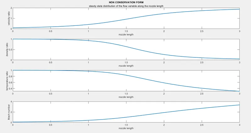
Steady-state distribution of primitive variables inside the nozzle for non-conservative form
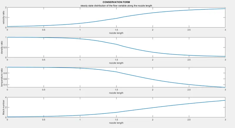
Steady-state distribution of primitive variables inside the nozzle for conservative form
Time-wise variation of the primitive variables
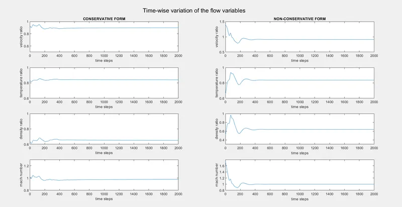
The above plots are the time wise variation of the flow variables both in the conservative form and the non-conservative form.
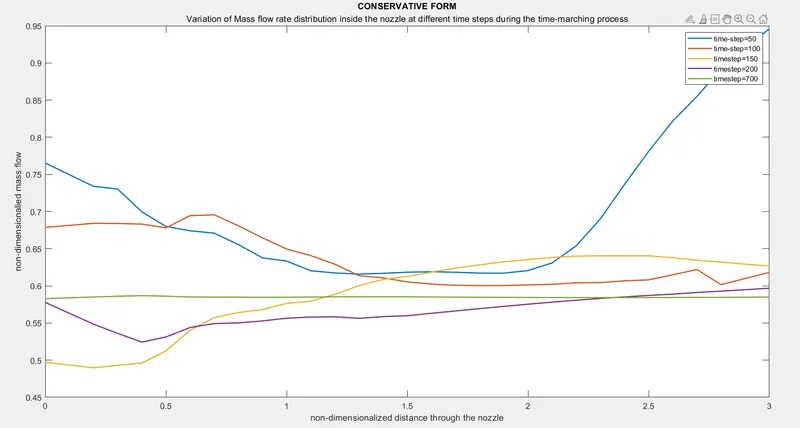
Variation of Mass flow rate distribution inside the nozzle at different time steps during the time-marching process
Conservative form
Non-conservative form
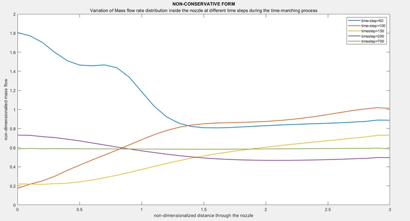
The above plots shows the non-dimensional mass flow as a function of the nondimensional distance through the nozzle. Each of the curve represents different time instances during the course of the time marching procedure. During the initial steps the variation in the mass flow rate is observed, but as the timestep reaches around 700, the curve is almost a straight line, it can be inferred that the mass flow has converged to a steady state value. Analytical calculating the mass flow rate steady state value is :
`rho*V*A = rho^**sqrtT^** = 0.579`.
In the above plots also, as the time steps increased, in can be noticed that the mass flow rate reaches this value.
Comparison of Normalized mass flow rate distributions of both forms
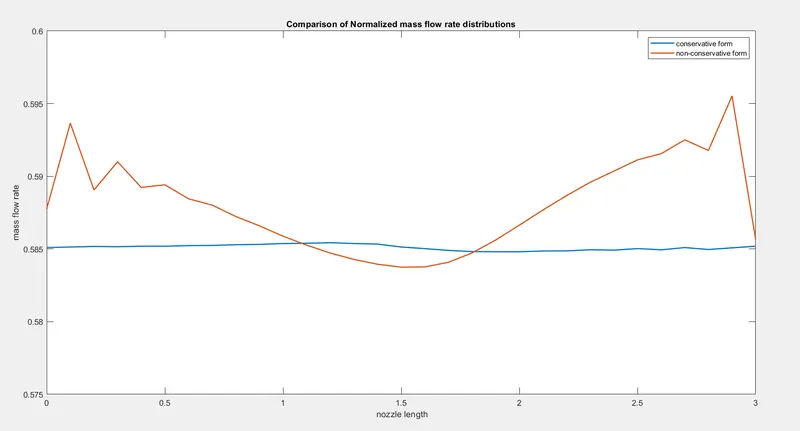
From the above plot regarding the mass flow rate across the nozzle length, it can be infer that the conservative form offers better results compared to the non-conservative form
Perform a grid independence test on the solution
To perform the grid independence test the number of grid points(currently 31) is increased upto almost twice the value and the values are compared, if the values are significantly different, then the number of grid points has to be increased to such a point that where the increase in the number of grid point doesnt affect the final solution.
For the grid independence the conservative and the non-conservative forms are solved initially with 31 grid points and then with 61 grid points. If the solutions are close, then the state is said to be grid independent. The steady state values of density, temperature, mach number and velocity at the throat will be compared with 31 grid points and 61 grid points.
Non-conservative form :
| Flow parameters | Grid points = 31 | Grid points = 61 |
| Density | 0.6389 | 0.6374 |
| Velocity | 0.9140 | 0.9138 |
| Temperature | 0.8365 | 0.8353 |
| Mach number | 0.9994 | 0.9998 |
Conservative form :
| Flow parameters | Grid points = 31 | Grid points = 61 |
| Density | 0.6517 | 0.6384 |
| Velocity | 0.8979 | 0.9130 |
| Temperature | 0.8407 | 0.8353 |
| Mach number | 0.9794 | 0.9990 |
It can be noticed that as the grid points increases, the values of the flow variables at the throat has no significant difference. Hence it can be concluded that both the conservative and the non-conservative form are grid independent.
Comparing both the non-conservative and the conservative forms, the following conclusions can be stated :
- There is no much difference in the steady state values of the conservative and the non-conservative forms. In terms of accuracy the non-conservative form tends to produce accurate values for the primitive variables like velocity, pressure and others. Whereas the conservative form gives accurate results for the flux variables.
- The residual decay is faster in the non-conservative form. The non-conservative form leads to smaller residuals. In that manner the non-conservative form does a better work in solving.
- The conservative form handles the normalized mass flow rate distribution across the nozzle much better, in other words the conservation form is able to conserve the mass better.
- The non-conservative form simulations are faster compared to the conservative form simulations.
- Both the conservative and the non-conservative forms are grid independent.
Reference :
Computational Fluid Dynamics - The basics with applications - By John.D.Anderson