CFD using MATLAB - Solving the steady and unsteady 2D heat conduction problem
Solving 2D Transient Heat conduction Equation
For an unsteady state the 2-D heat conduction equation is represented as :
`(delT)/(delt) = alpha*((del^2T)/(delx^2) + (del^2T)/(dely^2))`
For a steady state condition, the heat conduction equation is represented as :
`((del^2T)/(delx^2) + (del^2T)/(dely^2)) = 0`
These equation are partial differential equation, and hence the numerical discretization techniques can be used to solve these equations using the numerical analysis.
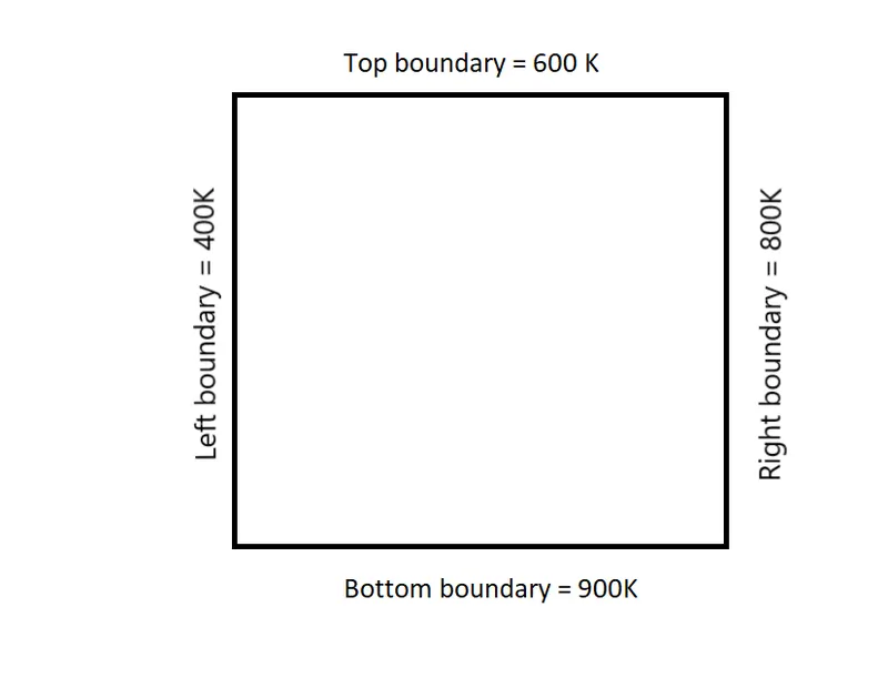
The boundary conditions for the problem are as given below :
For the transient analysis, either the equations can be solved in its implicit form or in its explicit form.
The `(delT)/(delt)` is discretized using the forward time marching scheme as `(T_(i,j)^(n+1) - T_(i,j)^n)/(Deltat)`.
The subscript (i,j) denotes the nodes and the superscript represents the time step.
Since the right hand side of the equation is a second order partial derivative, the central differencing scheme is used for discretizing the terms as follows :
`(del^2T)/(delx^2) = (T_(i-1,j) - 2*T_(i,j) + T_(i+1,j))/(Deltax^2)`
`(del^2T)/(dely^2) = (T_(i,j-1) - 2*T_(i,j) + T_(i,j+1))/(Deltay^2)`
Depending on which time step these second order derivated are computed, they can be termed as implicit and explicit.
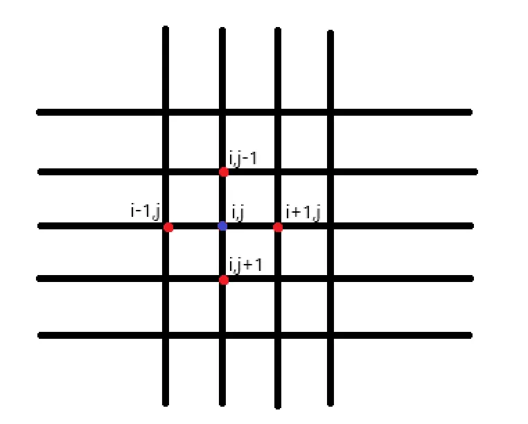
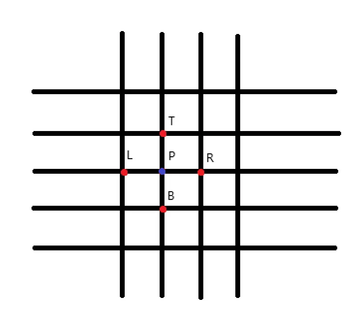
For simplicity, the subscripts are replaced as shown in the diagram :
Explicit form :
When computed at the previous time step `n`, the equation is of the explicit form.
`(T_p^(n+1) - T_p^n)/(Deltat) = alpha*[(T_L^n - 2*T_P^n + T_R^n)/(Deltax^2) + (T_T^n - 2*T_P^n + T_B^n)/(Deltay^2)]`
Rearranging,
`T_p^(n+1) = T_p^n + alpha*(Deltat)*[(T_L^n - 2*T_P^n + T_R^n)/(Deltax^2) + (T_T^n - 2*T_P^n + T_B^n)/(Deltay^2)]`
Lets consider `(alpha*(Deltat)) / (Deltax^2) = k_1` and `(alpha*(Deltat)) / (Deltay^2) = k_2``
Subtituting these values in the equation :
`T_p^(n+1) = T_p^n + k_1*(T_L^n - 2*T_P^n + T_R^n) + k_2*(T_T^n - 2*T_P^n + T_B^n)`
`T_p^(n+1) = T_p^n*[1-2*k_1-2*k_2] + k_1*(T_L^n + T_R^n) + k_2*(T_T^n + T_B^n)`
These equations can be used directly to compute the LHS, since all the values in the RHS is known.
Implicit form :
If the of the second order derivative terms are computed at the current time step (n+1), then the equation is of the implicit form.
`(T_p^(n+1) - T_p^n)/(Deltat) = alpha*[(T_L^(n+1) - 2*T_P^(n+1) + T_R^(n+1))/(Deltax^2) + (T_T^(n+1) - 2*T_P^(n+1) + T_B^(n+1))/(Deltay^2)]`
Rearranging,
`T_p^(n+1) = T_p^n + alpha*(Deltat)*[(T_L^(n+1) - 2*T_P^(n+1) + T_R^(n+1))/(Deltax^2) + (T_T^(n+1) - 2*T_P^(n+1) + T_B^(n+1))/(Deltay^2)]``
Lets consider `(alpha*(Deltat)) / (Deltax^2) = k_1` and `(alpha*(Deltat)) / (Deltay^2) = k_2``
Subtituting these values in the equation :
`T_p^(n+1) = T_p^n + k_1*(T_L^(n+1) - 2*T_P^(n+1) + T_R^(n+1)) + k_2*(T_T^(n+1) - 2*T_P^(n+1) + T_B^(n+1))`
`T_p^(n+1) =( T_p^n + k_1*(T_L^(n+1) + T_R^(n+1)) + k_2*(T_T^(n+1) + T_B^(n+1)))/(1+2*k_1+2*k_2)`
For implicit form of the equation the RHS is still unknown, therfore system of equations are converted to matrix form and then solved. In other ways the implicit form can also be solved using iterative solvers. The iterative solvers make guess for the unknown values and then compute the error value, and until the residual error comes below a specified limit, the guess values are modified using a transformation matrix and a constant. The residual error or otherwise called as the tolerance is specified by the user before the start of the iterations.
The various methods used by the iterative solvers are :
- Jacobi method :
Jacobi iterative method is considered as an iterative algorithm which is used for determining the solutions for the system of linear equations. In this method, an approximate value (guess) is used and then the entire equation is solved using this guess value. Until it converges, the process is iterated. With the Jacobi method, the values of `T_i^n`obtained in the `n^(th)` iteration remains unchanged until the entire `(n+1)^(th)` iteration has been calculated.
- Gauss Siedel method :
With the Gauss-Seidel method, we use the new values `T_i^(n+1)` as soon as they are known. For example,
once we have computed `T_1^(n+1)`from the first equation, its value is then used in the second equation to obtain the new `T_2^(n+1)` and so on.
In simpler words the difference between the Gauss–Seidel and Jacobi methods is that the Jacobi method uses the values obtained from the previous step while the Gauss–Seidel method always applies the latest updated values during the iterative procedures.
- Successive over relaxation (SOR) method :
This iterative method uses a value `omega` (omega) to guess the value for next iteration. By employing the below mentioned formula the values are computed.
`T_i^(n+1) = T_i^n*(1-omega) + omega*(T_(GS))`
In this `T_(GS)`is the value computed using the gauss-siedel iteration method formula. In this manner the gauss siedel method is extended to the relaxation methods.
Transient Analysis using the explicit scheme
Since the RHS is completely known, iterative solvers are not used. In this case for numerical discretization is done and the temperature at each node is calculated. The MATLAB program is as follows. The only parameter to be kept in check is the CFL indicated as `k_1 and k_2` in the program. The summation of both should be less than or equal to 0.5 for the analysis to be stable. In this case the CFL value is 0.4536.
CODE :
close all
clear all
clc

% input parameters
nx=10; % number of nodes in the x-direction
ny=10; % number of nodes in the y-direction
dt=0.002 ; % timestep
alpha = 1.4; % thermal diffusivity
nt = 500;   % number of timesteps

T = 300*ones(nx,ny);

% initial conditions
for i = 1:nx
    T(1,i) = 600;
    T(ny,i)=900;
end
for j=1:ny
    T(j,1) = 400;
    T(j,nx) = 800;
end
T(1,1)= (T(1,2)+ T(2,1))/2;
T(1,nx) = (T(1,nx-1)+T(2,nx))/2;
T(ny,1) = (T(ny-1,1) + T(ny,2))/2;
T(ny,nx) = (T(ny,nx-1)+T(ny-1,nx))/2;


%creating a 2D mesh
x = linspace(0,1,nx);
y = linspace(0,1,ny);
dx = x(2)-x(1);
dy = y(2)-y(1);

Told = T;

%CFL values for stability
k1 = alpha*(dt/(dx^2));
k2 = alpha*(dt/(dy^2));
CFL = k1+k2;

% Time loop
 for k = 1:nt

     for i=2:nx-1

        for j=2:ny-1

             T(i,j) = (Told(i,j) + (k1*(Told(i+1,j)-(2*Told(i,j))+Told(i-1,j))) + (k2*(Told(i,j-1)-(2*Told(i,j)) +Told(i,j+1))));
        end

     end
   Told = T;
   % plotting the heatmap for each iteration.
    colormap(jet);
    A=contourf(x,y,T);
    clabel(A);
    set(gca,'YDir','reverse');
    xlabel('X-Direction');
    ylabel('Y-Direction');
    grid on ;
    title (' Transient Analysis of 2D-heat conduction equation using explicit scheme');
    B = sprintf(' Number of timesteps = %d,  timestep (dt) = %d',k,dt);
    subtitle(B);
    pause(0.0001);
 end
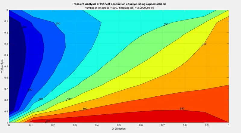
The plot is programmed in the time loop inorder to notice the changes in the temperature distribution at each timestep. The solution reaches a steady state even before the specified number of timesteps. If the timestep size(dt) is varied accordingly the time taken to reach the steady state will also vary. For the current timestep of 0.002 the solution reaches a steady state at around 100 to 150 iterations. Other than the timestep, even the node size and the alpha(thermal diffusivity) also affect the time taken to achieve a steady state.
OUTPUT :
Transient Analysis using the implicit scheme
In this case, since the RHS of the equation are unknown, the iterative solvers are used. The three iterative methods indicated above are used in the following MATLAB program.
CODE :
close all
clear all
clc

% input parameters
nx=10; % number of nodes in the x-direction
ny=10; % number of nodes in the y-direction
dt=0.0001 ; % timestep
alpha = 1.4; % thermal diffusivity
T = 300*ones(ny,nx);  % initial guess values for temperature


% initial conditions
for i = 1:nx
   T(1,i) = 600;
   T(ny,i)=900;
end
for j=1:ny
    T(j,1) = 400;
    T(j,nx) = 800;
end
T(1,1)= (T(1,2)+ T(2,1))/2;
T(1,nx) = (T(1,nx-1)+T(2,nx))/2;
T(ny,1) = (T(ny-1,1) + T(ny,2))/2;
T(ny,nx) = (T(ny,nx-1)+T(ny-1,nx))/2;

%creating a 2D mesh
x = linspace(0,1,nx);
y = linspace(0,1,ny);
dx = x(2)-x(1);
dy = y(2)-y(1);

Told = T;

% selection of the types of solver
iteration = 3;

% tolerance for convergence of temperture
tol = 1e-4;

k1 = alpha*(dt/(dx^2));
k2 = alpha*(dt/(dy^2));
Tprev = T;

iter = 1 ;

%Joacobi method
if iteration ==1

 for k=1:1500 % time loop

    error = 9e9;

    while(error > tol) % convergence loop

         for i=2:ny-1

            for j=2:nx-1

                term1 = (1/(1+(2*k1)+(2*k2)));
                term2 = k1*term1;
                term3 = k2*term1;
                T(i,j) = (term1*Tprev(i,j)) + (term2*(Told(i+1,j)+Told(i-1,j))) + (term3*(Told(i,j-1)+Told(i,j+1)));

            end

         end

        error = max(max(abs(Told-T))); % calculating maximum error value
        Told = T; % updating the old temperature values
        iter = iter +1;

    end

    Tprev = T;


 end
end


 %Gauss-siedel method
if iteration ==2

 for k=1:1500 % time loop

    error = 9e9;

    while(error > tol) % convergence loop

         for i=2:ny-1

            for j=2:nx-1

                term1 = (1/(1+(2*k1)+(2*k2)));
                term2 = k1*term1;
                term3 = k2*term1;
                T(i,j) = (term1*Tprev(i,j)) + (term2*(Told(i+1,j)+T(i-1,j))) + (term3*(T(i,j-1)+Told(i,j+1)));

            end

         end

        error = max(max(abs(Told-T))); % calculating error values
        Told = T; % updating the old temperature values
        iter = iter +1;

    end

    Tprev = T;

 end
end

%SOR method
if iteration ==3

    omega = 1.013; % Value of omega

 for k=1:1500 % time loop

    error = 9e9;

    while(error > tol) % convergence loop

         for i=2:ny-1

            for j=2:nx-1

                term1 = (1/(1+(2*k1)+(2*k2)));
                term2 = k1*term1;
                term3 = k2*term1;
                T(i,j) = ((1-omega)*Told(i,j)) + omega*((term1*Tprev(i,j)) + (term2*(Told(i+1,j)+T(i-1,j))) + (term3*(T(i,j-1)+Told(i,j+1))));

            end

         end

        error = max(max(abs(Told-T))); % calculating error value
        Told = T; % updating the old temperature values
        iter = iter +1;

    end

    Tprev = T;

 end
end

% plotting the temperature distribution
    figure(1)
    colormap(jet);
    A=contourf(x,y,T);
    clabel(A);
    set(gca,'YDir','reverse');
    xlabel('X-Direction');
    ylabel('Y-Direction');
    grid on ;
    title(' Transient analysis of 2D heat equation using implicit scheme(Jacobi method)');
    B = sprintf('number of timestep = %d , Number of iteration = %d',k,iter);
    subtitle(B);
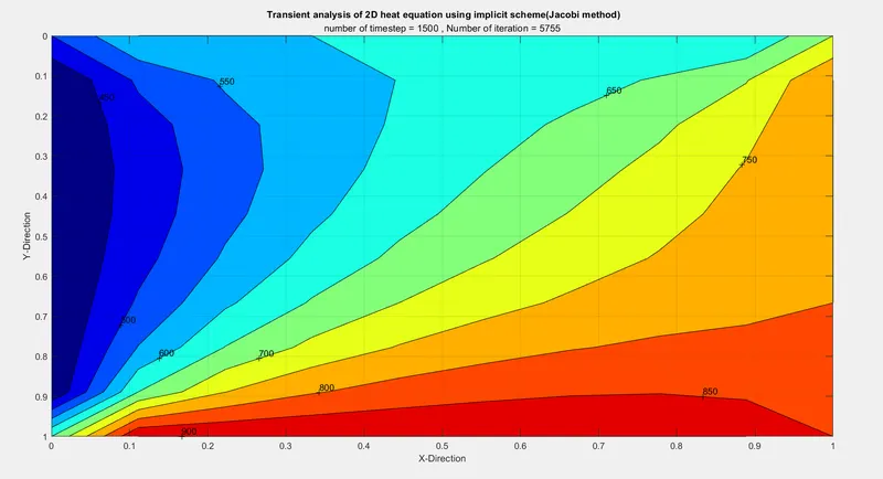
In the code, all the three iterative solvers are used. The parameter 'iteration' is used to select solver solver. iteration=1 is the iterative solver which uses the jacobi method. iteration=2 is the iterative solver which uses the gauss siedel method and hte iterative solver=3, uses the successive over relaxation method.
The formulas and the output temperature distribution for various methods is given below :
Jacobi method
Formula :
`T_p^(n+1) = (T(prev)_p^n + k_1*(T(old)_R^(n+1) + T(old)_L^(n+1)) + k_2*(T(old)_T^(n+1) + T(old)_B^(n+1)))/(1+2*k_1 + 2*k_2)`
The `T(old)` represent the guess values from the previous iteration. These values are updated after every iteration and not within an iteration. The `T(prev)` represents the temperature values from the previous timestep. It remains constant at a particular time step. The other variables to be noted are the CFL factors :
`k_1 = (alpha*Deltat)/(Deltax^2)` and `k_2 = (alpha*Deltat)/(Deltay^2)`
Output plot :
Gauss-siedel method
Formula :
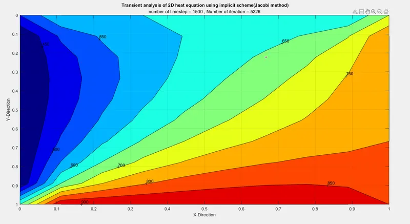
`T_p^(n+1) = (T(prev)_p^n + k_1*(T(old)_R^(n+1) + T_L^(n+1)) + k_2*(T_T^(n+1) + T(old)_B^(n+1)))/(1+2*k_1 + 2*k_2)`
In this case the left point and the top point values are calculated in the iteration and guess value is updated within an iteration, Whereas in jacobi the old guess values are used and hence are not updated within an iteration.
Output Plot :
Successive over relaxation method
Formula :
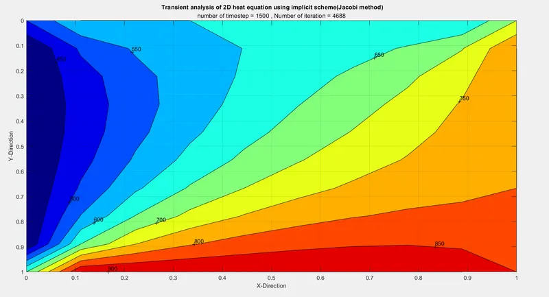
`T_p^(n+1) = (1-omega)*T(old)_p^n + omega*((T(prev)_p^n + k_1*(T(old)_R^(n+1) + T(old)_L^(n+1)) + k_2*(T(old)_T^(n+1) + T(old)_B^(n+1)))/(1+2*k_1 + 2*k_2))`
The `omega` is the relaxation factor.
Output Plot :
The number of iterations is as follows :
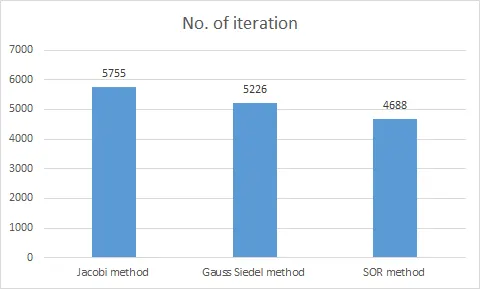
This data is based on running the iterative solver for 1500 timesteps, with each timestep of 0.0001 seconds. The trend in terms of the number of iteration for convergence is :
Jacobi method > Gauss-siedel method > SOR method.
Steady state analysis of 2D heat conduction problem
For a steady state condition, the heat conduction equation is represented as :
`((del^2T)/(delx^2) + (del^2T)/(dely^2)) = 0`
CODE :
close all
clear all
clc

% input parameters
nx=10; % number of nodes in the x-direction
ny=10; % number of nodes in the y-direction
dt=1e-4 ; % timestep size
alpha = 1.4; % thermal diffusivity


T = 300*ones(nx,ny);
% initial conditions
for i = 1:nx
    T(1,i) = 600;
    T(ny,i)=900;
end
for j=1:ny
    T(j,1) = 400;
    T(j,nx) = 800;
end
T(1,1)= (T(1,2)+ T(2,1))/2;
T(1,nx) = (T(1,nx-1)+T(2,nx))/2;
T(ny,1) = (T(ny-1,1) + T(ny,2))/2;
T(ny,nx) = (T(ny,nx-1)+T(ny-1,nx))/2;

%creating a 2D mesh
x = linspace(0,1,nx);
y = linspace(0,1,ny);

dx = x(2)-x(1);
dy = y(2)-y(1);

Told = T;

% selection of the iterative solver method
iteration = 1;

% tolerance for convergence of temperture
tol = 1e-4;
error = 1e4;

k = ((2*(dy^2 + dx^2))/(dy^2*dx^2));

%Jacobi method
if iteration == 1
   iter = 1 ;

    while(error > tol)

    for i=2:nx-1

        for j=2:ny-1

            term_1 = ((Told(i+1,j) + Told(i-1,j))/(k*dx^2));
            term_2 = ((Told(i,j-1) + Told(i,j+1))/(k*dy^2));
            T(i,j) = term_1 + term_2;

        end

    end

    error = max(max(abs(Told-T)));
    Told = T;
    iter = iter +1;

    end
end


%Gauss-siedel method

if iteration == 2

   iter = 1 ;

    while(error > tol)

    for i=2:nx-1

        for j=2:ny-1

            term_1 = ((Told(i+1,j) + T(i-1,j))/(k*dx^2));
            term_2 = ((T(i,j-1) + Told(i,j+1))/(k*dy^2));
            T(i,j) = term_1 + term_2;

        end

    end

    error = max(max(abs(Told-T)));
    Told = T;
    iter = iter +1;

    end

end


%succesive over-relaxation method

omega=1.5;

if iteration == 3

   iter = 1 ;

    while(error > tol)

    for i=2:nx-1

        for j=2:ny-1

            term_1 = ((Told(i+1,j) + T(i-1,j))/(k*dx^2));
            term_2 = ((T(i,j-1) + Told(i,j+1))/(k*dy^2));
            T(i,j) = ((Told(i,j)*(1-omega)) + omega*(term_1 + term_2));

        end

    end

    error = max(max(abs(Told-T)));
    Told = T;
    iter = iter +1;

    end

end

% plotting the temperature distribution
figure(1)
colormap(jet);
A=contourf(x,y,T);
clabel(A);
set(gca,'YDir','reverse');
xlabel('X-Direction');
ylabel('Y-Direction');
grid on ;
title('Steady State Analysis of 2D Heat conduction');
B = sprintf('Iterative method = %d , Number of iterations = %d , Error = %d',iteration,iter,error);
subtitle(B);
This code uses three iterative solvers to solve the PDE. The parameter 'iteration' is used to select solver solver. iteration=1 is the iterative solver which uses the jacobi method. iteration=2 is the iterative solver which uses the gauss siedel method and hte iterative solver=3, uses the successive over relaxation method.
Since its a steady state the time loop is not found as in the case of the unsteady analysis code. Since its a steady state equation the formula also changes.
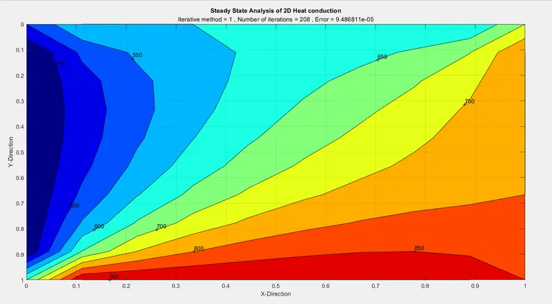
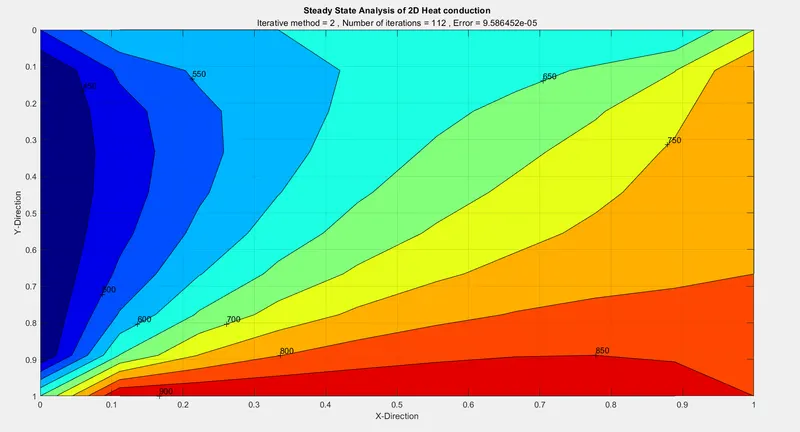
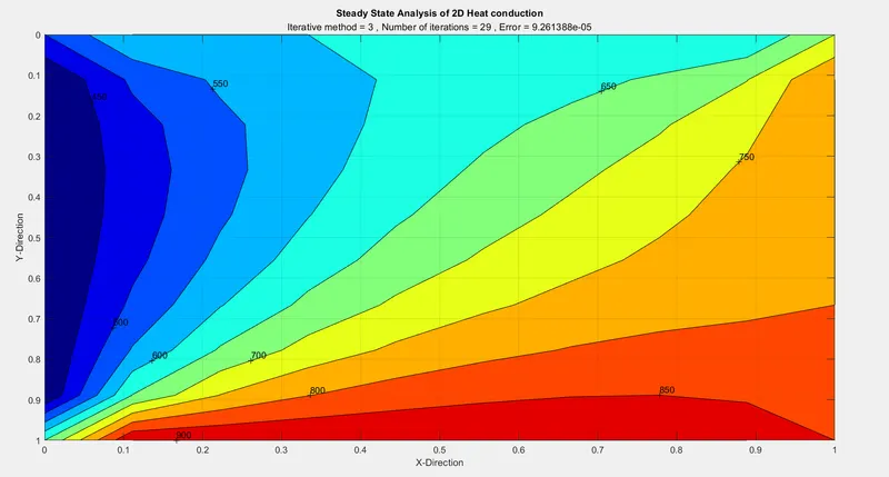
The formulas and the output plot when the three iterative solvers are used are as shown.
Jacobi method
Formula :
`T_p = 1/k*[((T(old)_R + T(old)_L)/(Deltax^2)) + ((T(old)_T + T(old)_B)/(Deltay^2))]`
Where `k = 2*((Deltax^2 + Deltay^2)/(Deltax^2*Deltay^2))`
Output Plot :
Gauss-Siedel method
Formula :
`T_p = 1/k*[((T(old)_R + T_L)/(Deltax^2)) + ((T_T + T(old)_B)/(Deltay^2))]`
Output Plot :
Successive over relaxation (SOR) method
Formula :
`T_p = (1-omega)*T(old)_p + omega*(1/k*[((T(old)_R + T_L)/(Deltax^2)) + ((T_T + T(old)_B)/(Deltay^2))])`
In this case, the relaxation factor `(omega)` is kept at 1.5. It is at this value that the number of iteration required to attain convergence is minimum.
Output Plot :
The number of iterations required to reach convergence is as follows :
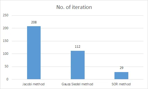
It can be concluded that the number of iteration required is least in SOR method. The maximum number of iteration is seen in jacobi method. So, the trend in terms of the number of iteration for convergence is :
Jacobi method > Gauss-siedel method > SOR method.