Deriving 4th order approximation of a 2nd order derivative using Taylor Table method
Derive the following 4th order approximations of the second-order derivative.
1. Central difference
2. Skewed right-sided difference
3. Skewed left-sided difference
To compute the second order derivative, say `(del^2phi)/dx^2` with fourth order approximation, taylor table can be used.
Central differencing scheme
Derivation :
First the number of nodes that should be considered is calculated. For central differencing scheme the formula for the number of nodes is given by:
No. of nodes = p+q-1
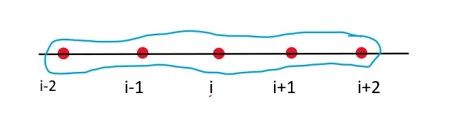
Where p is the order of the derivative , q is the order of approximation. In this case p=2 and q=4, thus the number of nodes to be taken into consideration is 5. To compute it using the central difference scheme, the points `i-2 , i-1, i, i+1, i+2` is considered. as shown in the figure below.
Consider the equation to be :
`Deltax^2*(del^2f)/dx^2 = a*f(i-2) + b*f(i-1) + c*f(i) + d*f(i+1) + e*f(i+2)`
pplying the taylor series expansion for the all the points ,
`a*f(i-2) = a*[ f(i) - ((2*Deltax*f'(i))/(1!)) + ((4*Deltax^2*f''(i))/(2!)) - ((8*Deltax^3*f'''(i))/(3!)) + ((16*Deltax^4*f''''(i))/(4!)) - ((32*Deltax^5*f'''''(i))/(5!)) + O[Deltax^6]]`
`b*f(i-1) = b*[ f(i) - ((Deltax*f'(i))/(1!)) + ((Deltax^2*f''(i))/(2!)) - ((Deltax^3*f'''(i))/(3!)) + ((Deltax^4*f''''(i))/(4!)) - ((Deltax^5*f'''''(i))/(5!)) + O[Deltax^6]]`
`c*f(i) = c*f(i)`
`e*f(i+2) = e*[ f(i) + ((2*Deltax*f'(i))/(1!)) + ((4*Deltax^2*f''(i))/(2!)) + ((8*Deltax^3*f'''(i))/(3!)) + ((16*Deltax^4*f''''(i))/(4!)) + ((32*Deltax^5*f'''''(i))/(5!)) + O[Deltax^6]]`
`d*f(i+1) = d*[ f(i) + ((Deltax*f'(i))/(1!)) + ((Deltax^2*f''(i))/(2!)) + ((Deltax^3*f'''(i))/(3!)) + ((Deltax^4*f''''(i))/(4!)) + ((Deltax^5*f'''''(i))/(5!)) + O[Deltax^6]]`
Adding both the LHS and the RHS we get :
On the LHS : `a*f(i-2) + b*f(i-1) + c*f(i) + d*f(i+1) + e*f(i+2)`` , which based on the initial equation is equal to `Deltax^2*(del^2f)/dx^2.`
On the RHS : `f(i) * [ a+b+c+d+e] + f'(i)*[-2aDeltax -bDeltax + dDeltax + 2eDeltax]`
`+ f''(i)* [((4Deltax^2*a)/2) + ((Deltax^2*b)/2) + ((Deltax^2*d)/2) + ((4Deltax^2*e)/2)]`
`+ f'''(i) * [ -((8Deltax^3*a)/6) - ((Deltax^3*b)/6) + ((Deltax^3*d)/6) + ((8*Deltax^3*e)/6)]`
`+ f''''(i)*[((16Deltax^4*a)/24) + ((Deltax^4*b)/24) + ((Deltax^4*d)/24) + ((16Deltax^4*e)/24)]`
`+ f'''''(i)*[-((32Deltax^5*a)/120) - ((Deltax^5*b)/120) + ((Deltax^5*d)/120) + ((32Deltax^5*e)/120)]`
`+ O[Deltax^6]`
Based on the equations, the following taylors table can be drawn :
| `f(i)` | `Deltax*f'(i)` | `Deltax^2*f''(i)` | `Deltax^3*f'''(i)` | `Deltax^4*f''''(i)` | `(Deltax^5*f'''''(i)` | |
| `a*f(i-2)` | `a` | `-2a` | `(4a)/2` | `-(8a)/6` | `(16a)/24` | `-(32a)/120` |
| `b*f(i-1)` | `b` | `-b` | `b/2` | `-b/6` | `b/24` | `-b/120` |
| `c*f(i)` | `c` | `0` | `0` | `0` | `0` | `0` |
| `d*f(i+1)` | `d` | `d` | `d/2` | `d/6` | `d/24` | `d/120` |
| `e*f(i+2)` | `e` | `2e` | `(4e)/2` | `(8e)/6` | `(16e)/24` | `(32e)/120` |
| `0` | `0` | `1` | `0` | `0` |
This taylor table gives a matrix form of the equation, which can be solved in MATLAB.
The matrix form of the equations is :
`[[1,1,1,1,1],[-2,-1,0,1,2],[4/2,1/2,0,1/2,4/2],[-8/6,-1/6,0,1/6,8/6],[16/24,1/24,0,1/24,16/24]]*[[a],[b],[c],[d],[e]] = [[0],[0],[1],[0],[0]]`
Solving this, the coefficient is obtained and then substituted into the main equation, using which the second order derivative can be calculated numerically with the fourth order approximation.
The solution is as follows :
`[[a],[b],[c],[d],[e]] = [[-0.0833],[1.3333],[-2.5000],[1.3333],[-0.0833]]`
The equation is :
`(del^2f)/dx^2 = [(-0.08333*f(i-2) + 1.3333*f(i-1) - 2.5*f(i) + 1.333*f(i+1) - 0.08333e*f(i+2))/(Deltax^2)]`
Skewed right-sided differencing scheme
Derivation :
The number of nodes that should be considered is calculated based on the below mentioned formula. For skewed right-sided differencing scheme the formula for the number of nodes is given by:
No. of nodes = p+q
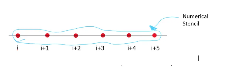
Where p is the order of the derivative , q is the order of approximation. In this case p=2 and q=4, thus the number of nodes to be taken into consideration is 6. To compute it using the skewed right-sided difference scheme, the points ` i, i+1, i+2, i+3, i+4, i+5` is considered. as shown in the figure below.`
Consider the equation to be :
`Deltax^2*(del^2f)/dx^2 = a*f(i) + b*f(i+1) + c*f(i+2) + d*f(i+3) + e*f(i+4) + g*f(i+5)`
Applying the taylor series expansion for the all the points ,
`a*f(i) = a*f(i)`
`b*f(i+1) = b*[ f(i) + ((Deltax*f'(i))/(1!)) + ((Deltax^2*f''(i))/(2!)) + ((Deltax^3*f'''(i))/(3!)) + ((Deltax^4*f''''(i))/(4!)) + ((Deltax^5*f'''''(i))/(5!)) + O[Deltax^6]]`
`c*f(i+2) = c*[ f(i) + ((2*Deltax*f'(i))/(1!)) + ((4*Deltax^2*f''(i))/(2!)) + ((8*Deltax^3*f'''(i))/(3!)) + ((16*Deltax^4*f''''(i))/(4!)) + ((32*Deltax^5*f'''''(i))/(5!)) + O[Deltax^6]]`
`d*f(i+3) = d*[ f(i) + ((3Deltax*f'(i))/(1!)) + ((9Deltax^2*f''(i))/(2!)) + ((27Deltax^3*f'''(i))/(3!)) + ((81Deltax^4*f''''(i))/(4!)) + ((243Deltax^5*f'''''(i))/(5!)) + O[Deltax^6]]`
`e*f(i+4) = e*[ f(i) + ((4Deltax*f'(i))/(1!)) + ((16Deltax^2*f''(i))/(2!)) + ((64Deltax^3*f'''(i))/(3!)) + ((256Deltax^4*f''''(i))/(4!)) + ((1024Deltax^5*f'''''(i))/(5!)) + O[Deltax^6]]`
`g*f(i+5) = g*[ f(i) + ((5Deltax*f'(i))/(1!)) + ((25Deltax^2*f''(i))/(2!)) + ((125Deltax^3*f'''(i))/(3!)) + ((625Deltax^4*f''''(i))/(4!)) + ((3125Deltax^5*f'''''(i))/(5!)) + O[Deltax^6]]`
Adding both the LHS and the RHS we get :
In the LHS : `a*f(i) + b*f(i+1) + c*f(i+2) + d*f(i+3) + e*f(i+4) + g*f(i+5)`, which based on the initial equation is equal to`Deltax^2*(del^2f)/dx^2.`
On the RHS : `f(i) * [ a+b+c+d+e+g] + f'(i)*[bDeltax + 2cDeltax + 3dDeltax + 4eDeltax + 5gDeltax]`
`+ f''(i)* [((Deltax^2*b)/2) + ((4Deltax^2*c)/2) + ((9Deltax^2*d)/2) + ((16Deltax^2*e)/2)+((25Deltax^2*g)/2)]`
`+ f'''(i) * [ ((Deltax^3*b)/6) + ((8Deltax^3*c)/6) + ((27Deltax^3*d)/6) + ((64*Deltax^3*e)/6) + ((125*Deltax^3*g)/6)]`
`+ f''''(i)*[((Deltax^4*b)/24) + ((16*Deltax^4*c)/24) + ((81*Deltax^4*d)/24) + ((256*Deltax^4*e)/24) + ((625*Deltax^4*g)/24)]`
`+ f'''''(i)*[((Deltax^5*b)/120) + ((32*Deltax^5*c)/120) + ((243*Deltax^5*d)/120) + ((1024*Deltax^5*e)/120) + ((3125*Deltax^5*g)/120)]`
`+ O[Deltax^6]`
Based on the equations, the following taylors table can be drawn :
| `f(i)` | `Deltax*f'(i)` | `Deltax^2*f''(i)` | `Deltax^3*f'''(i)` | `Deltax^4*f''''(i)` | `(Deltax^5*f'''''(i)` | |
| `a*f(i)` | `a` | `0` | `0` | `0` | `0` | `0` |
| `b*f(i+1)` | `b` | `b` | `b/2` | `b/6` | `b/24` | `b/120` |
| `c*f(i+2)` | `c` | `2c` | `(4c)/2` | `(8c)/6` | `(16c)/24` | `(32c)/120` |
| `d*f(i+3)` | `d` | `3d` | `(9d)/2` | `(27d)/6` | `(81d)/24` | `(243d)/120` |
| `e*f(i+4)` | `e` | `4e` | `(16e)/2` | `(64e)/6` | `(256e)/24` | `(1024e)/120` |
| `g*f(i+5)` | `g` | `5g` | `(25g)/2` | `(125g)/6` | `(625g)/24` | `(3125g)/120` |
This taylor table gives a matrix form of the equation, which can be solved in MATLAB.
The matrix form of the equations is :
`[[1,1,1,1,1,1],[0,1,2,3,4,5],[0,1/2,4/2,9/2,16/2,25/2],[0,1/6,8/6,27/6,64/6,125/6],[0,1/24,16/24,81/24,256/24,625/24],[0,1/120,32/120,243/120,1024/120,3125/120]]*[[a],[b],[c],[d],[e],[f]] = [[0],[0],[1],[0],[0],[0]]`
Solving this, the coefficient is obtained and then substituted into the main equation, using which the second order derivative can be calculated numerically with the fourth order approximation.
The solution is as follows :
`[[a],[b],[c],[d],[e],[g]] = [[3.7500],[-12.8333],[17.8333],[-13.0000],[5.0833],[-0.8333]]`
The equation is :
`(del^2f)/dx^2 = [(3.75*f(i) - 12.8333*f(i+1) + 17.8333*f(i+2) - 13.00*f(i+3) + 5.0833e*f(i+4) - 0.8333f(i+5))/(Deltax^2)]`
Skewed right-sided differencing scheme
Derivation :
The number of nodes is calculated based on the following formula. For skewed left-sided differencing scheme the formula for the number of nodes is given by:
No. of nodes = p+q
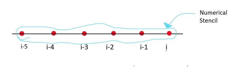
Where p is the order of the derivative , q is the order of approximation. In this case p=2 and q=4, thus the number of nodes to be taken into consideration is 6. To compute it using the skewed left-sided difference scheme, the points ` i, i-1, i-2, i-3, i-4, i-5` is considered. as shown in the figure below.`
Consider the equation to be :
`Deltax^2*(del^2f)/dx^2 = a*f(i) + b*f(i-1) + c*f(i-2) + d*f(i-3) + e*f(i-4) + g*f(i-5)`
Applying the taylor series expansion for the all the points ,
`a*f(i) = a*f(i)`
`b*f(i-1) = b*[ f(i) - ((Deltax*f'(i))/(1!)) + ((Deltax^2*f''(i))/(2!)) - ((Deltax^3*f'''(i))/(3!)) + ((Deltax^4*f''''(i))/(4!)) - ((Deltax^5*f'''''(i))/(5!)) + O[Deltax^6]]`
`c*f(i-2) = c*[ f(i) - ((2*Deltax*f'(i))/(1!)) + ((4*Deltax^2*f''(i))/(2!)) - ((8*Deltax^3*f'''(i))/(3!)) + ((16*Deltax^4*f''''(i))/(4!)) - ((32*Deltax^5*f'''''(i))/(5!)) + O[Deltax^6]]`
`d*f(i-3) = d*[ f(i) - ((3Deltax*f'(i))/(1!)) + ((9Deltax^2*f''(i))/(2!)) - ((27Deltax^3*f'''(i))/(3!)) + ((81Deltax^4*f''''(i))/(4!)) - ((243Deltax^5*f'''''(i))/(5!)) + O[Deltax^6]]`
`e*f(i-4) = e*[ f(i) - ((4Deltax*f'(i))/(1!)) + ((16Deltax^2*f''(i))/(2!)) - ((64Deltax^3*f'''(i))/(3!)) + ((256Deltax^4*f''''(i))/(4!)) - ((1024Deltax^5*f'''''(i))/(5!)) + O[Deltax^6]]`
`g*f(i-5) = g*[ f(i) - ((5Deltax*f'(i))/(1!)) + ((25Deltax^2*f''(i))/(2!)) - ((125Deltax^3*f'''(i))/(3!)) + ((625Deltax^4*f''''(i))/(4!)) - ((3125Deltax^5*f'''''(i))/(5!)) + O[Deltax^6]]`
Adding both the LHS and the RHS we get :
In the LHS : `a*f(i) + b*f(i-1) + c*f(i-2) + d*f(i-3) + e*f(i-4) + g*f(i-5)` which based on the initial equation is equal to`Deltax^2*(del^2f)/dx^2.`
On the RHS : `f(i) * [ a+b+c+d+e+g] - f'(i)*[bDeltax + 2cDeltax + 3dDeltax + 4eDeltax + 5gDeltax]`
`+ f''(i)* [((Deltax^2*b)/2) + ((4Deltax^2*c)/2) + ((9Deltax^2*d)/2) + ((16Deltax^2*e)/2)+((25Deltax^2*g)/2)]`
`- f'''(i) * [ ((Deltax^3*b)/6) + ((8Deltax^3*c)/6) + ((27Deltax^3*d)/6) + ((64*Deltax^3*e)/6) + ((125*Deltax^3*g)/6)]`
`+ f''''(i)*[((Deltax^4*b)/24) + ((16*Deltax^4*c)/24) + ((81*Deltax^4*d)/24) + ((256*Deltax^4*e)/24) + ((625*Deltax^4*g)/24)]`
`- f'''''(i)*[((Deltax^5*b)/120) + ((32*Deltax^5*c)/120) + ((243*Deltax^5*d)/120) + ((1024*Deltax^5*e)/120) + ((3125*Deltax^5*g)/120)]`
`+ O[Deltax^6]`
Based on the equations, the following taylors table can be drawn :
| `f(i)` | `Deltax*f'(i)` | `Deltax^2*f''(i)` | `Deltax^3*f'''(i)` | `Deltax^4*f''''(i)` | `(Deltax^5*f'''''(i)` | |
| `a*f(i)` | `a` | `0` | `0` | `0` | `0` | `0` |
| `b*f(i+1)` | `b` | `-b` | `b/2` | `-b/6` | `b/24` | `-b/120` |
| `c*f(i+2)` | `c` | `-2c` | `(4c)/2` | `-(8c)/6` | `(16c)/24` | `-(32c)/120` |
| `d*f(i+3)` | `d` | `-3d` | `(9d)/2` | `-(27d)/6` | `(81d)/24` | `-(243d)/120` |
| `e*f(i+4)` | `e` | `-4e` | `(16e)/2` | `-(64e)/6` | `(256e)/24` | `-(1024e)/120` |
| `g*f(i+5)` | `g` | `-5g` | `(25g)/2` | `-(125g)/6` | `(625g)/24` | `-(3125f)/120` |
This taylor table gives a matrix form of the equation, which can be solved in MATLAB.
The matrix form of the equations is :
`[[1,1,1,1,1,1],[0,-1,-2,-3,-4,-5],[0,1/2,4/2,9/2,16/2,25/2],[0,-1/6,-8/6,-27/6,-64/6,-125/6],[0,1/24,16/24,81/24,256/24,625/24],[0,-1/120,-32/120,-243/120,-1024/120,-3125/120]]*[[a],[b],[c],[d],[e],[g]] = [[0],[0],[1],[0],[0],[0]]`
Solving this, the coefficient is obtained and then substituted into the main equation, using which the second order derivative can be calculated numerically with the fourth order approximation.
The solution is as follows :
`[[a],[b],[c],[d],[e],[g]] = [[3.7500],[-12.8333],[17.8333],[-13.0000],[5.0833],[-0.8333]]`
The equation is :
`(del^2f)/dx^2 = [(3.75*f(i) - 12.8333*f(i+1) + 17.8333*f(i+2) - 13.00*f(i+3) + 5.0833e*f(i+4) - 0.8333f(i+5))/(Deltax^2)]`
Write a program in Matlab to evaluate the second-order derivative of the analytical function exp(x)*cos(x) and compare it with the 3 numerical approximations.
Code:
close all
clear all
clc

% function to be evaluated is exp(x)* cos(x).

% Analytical solution is : f''(x) = -2*exp(x)*sin(x)

x= pi/3;
dx= linspace(pi/4, pi/400,100);

analytical = -2*exp(x)*sin(x) ;

% solving for coefficient

% central difference scheme
A1= [1,1,1,1,1;-2,-1,0,1,2;4/2,1/2,0,1/2,4/2;-8/6,-1/6,0,1/6,8/6;16/24,1/24,0,1/24,16/24];
B1 = [0;0;1;0;0];
X1 = linsolve(A1,B1);
% coefficients
a1 = X1(1);
b1 = X1(2);
c1 = X1(3);
d1 = X1(4);
e1 = X1(5);

% skewed right-sided difference scheme
A2= [1,1,1,1,1,1;0,1,2,3,4,5;0,1/2,4/2,9/2,16/2,25/2;0,1/6,8/6,27/6,64/6,125/6;0,1/24,16/24,81/24,256/24,625/24;0,1/120,32/120,243/120,1024/120,3125/120];
B2 = [0;0;1;0;0;0];
X2 = linsolve(A2,B2);
% coefficients
a2 = X2(1);
b2 = X2(2);
c2 = X2(3);
d2 = X2(4);
e2 = X2(5);
f2 = X2(6);

% skewed left-sided difference scheme
A3= [1,1,1,1,1,1;0,-1,-2,-3,-4,-5;0,1/2,4/2,9/2,16/2,25/2;0,-1/6,-8/6,-27/6,-64/6,-125/6;0,1/24,16/24,81/24,256/24,625/24;0,-1/120,-32/120,-243/120,-1024/120,-3125/120];
B3 = [0;0;1;0;0;0];
X3 = linsolve(A3,B3);
% coefficients
a3 = X3(1);
b3 = X3(2);
c3 = X3(3);
d3 = X3(4);
e3 = X3(5);
f3 = X3(6);


for i=1:length(dx)

% center difference scheme terms
T11(i) = (exp(x-(2*dx(i))))*(cos(x-(2*dx(i))));
T12(i) = (exp(x-dx(i)))*(cos(x-dx(i)));
T13(i) = exp(x)*cos(x);
T14(i) = (exp(x+dx(i)))*(cos(x+dx(i)));
T15(i) = (exp(x+(2*dx(i))))*(cos(x+(2*dx(i))));

solution1(i) = ((a1*T11(i)) + (b1*T12(i)) + (c1*T13(i)) + (d1*T14(i)) + (e1*T15(i)))/(dx(i)*dx(i));
Error1(i) = abs(analytical - solution1(i));


% skewed right-sided difference scheme terms
T21(i) = exp(x)*cos(x);
T22(i) = (exp(x+dx(i)))*(cos(x+dx(i)));
T23(i) = (exp(x+(2*dx(i))))*(cos(x+(2*dx(i))));
T24(i) = (exp(x+(3*dx(i))))*(cos(x+(3*dx(i))));
T25(i) = (exp(x+(4*dx(i))))*(cos(x+(4*dx(i))));
T26(i) = (exp(x+(5*dx(i))))*(cos(x+(5*dx(i))));

solution2(i) = ((a2*T21(i)) + (b2*T22(i)) + (c2*T23(i)) + (d2*T24(i)) + (e2*T25(i)) + (f2*T26(i)))/(dx(i)*dx(i));
Error2(i) = abs(analytical - solution2(i));


% skewed left-sided difference scheme terms
T31(i) = exp(x)*cos(x);
T32(i) = (exp(x-dx(i)))*(cos(x-dx(i)));
T33(i) = (exp(x-(2*dx(i))))*(cos(x-(2*dx(i))));
T34(i) = (exp(x-(3*dx(i))))*(cos(x-(3*dx(i))));
T35(i) = (exp(x-(4*dx(i))))*(cos(x-(4*dx(i))));
T36(i) = (exp(x-(5*dx(i))))*(cos(x-(5*dx(i))));

solution3(i) = ((a3*T31(i)) + (b3*T32(i)) + (c3*T33(i)) + (d3*T34(i)) + (e3*T35(i)) + (f3*T36(i)))/(dx(i)*dx(i));
Error3(i) = abs(analytical - solution3(i));

end

figure(1)
loglog(dx,Error1,'linewidth',3);
hold on;
loglog(dx,Error2,'linewidth',3);
hold on;
loglog(dx,Error3,'linewidth',3);
title('Absolute error comparison between various schemes','FontSize',25);
xlabel('dx (grid spacing)','FontSize',20);
ylabel('Absolute error','FontSize',20);
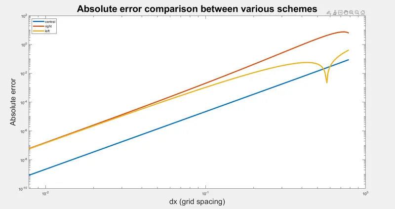
legend ('central','right','left','location','northwest');
Result :
Inference :
It can be inferred from the plot above that the absolute error of the central differencing scheme is less when compared to the skewed differencing schemes. The absolute error of the skewed right and left sided schemes are almost the same for most part. Hence the central differencing scheme can be inferred to be more accurate than the skewed schemes.
describe why a skewed scheme is useful? What can a skewed scheme do that a CD scheme cannot?
Skewed differencing schemes are better when the information from only one direction is available. The central differencing schemes requires information from all directions to compute the result. The skewed differencing schemes required information from only one direction. This can be required in case of the boundary problems. In the boundary information is present only from one side and in such cases skewed differencing schemes are preffered.