Assessment of road quality using Power Spectral Density (PSD) data

Road Surface Roughness :

The road surface roughness profile is also called as the elevation profile. Since the road profile data are random, we cannot use standard mathematical equations to represent the profile. One of the useful method of representation of the road profile is through power spectral density (PSD) which is essentially a plot of the signal power versus the spatial frequency. The ISO has proposed a road roughness classification based on the power spectral density. So, generally to determine the quality of the road or the road roughness, the road PSD profile data is taken and overlapped on the ISO standard road roughness class bands. From that plot we can infer the details regarding the quality of the road.

Octave Script

% road roughness classification 

clear all;
close all ;
clc;

% Road data
% The road data is loaded into the script
PSD=fopen('PSD_Data');

% obtaining the frequency data
% the first and last value are extracted seperated, because the line containing these values also have character data types.
first_line1 = fgetl(PSD);
first_value1 = first_line1(9:end);
frequency(1)=str2double(first_value1); 
for k=2:124
values1 = fgetl(PSD);
frequency(k) = str2double(values1); % frequency in cycle/ft
end 
last_line1 = fgetl(PSD);
last_value1 = last_line1(1:end-2);
frequency(125) = str2double(last_value1);

% obtaining the amplitude data
% the first and last value are extracted seperated, because the line containing these values also have character data types.
zero_line = fgetl(PSD);
first_line2 = fgetl(PSD);
first_value2 = first_line2(14:end);
amplitude(1)=str2double(first_value2);
for l=2:124
values2 = fgetl(PSD);
amplitude(l) = str2double(values2); % amplitude in ft^2/cycle/ft 
end 
last_value2 = fgetl(PSD);
amplitude(125) = str2double(last_value2);


% three frequencies (cycles/m)
omega(1) = 0.01;
omega(2) = 1/(2*pi);
omega(3) = 10;

%Generate road roughenss class lines
s_a(2) = 8e-6 ; %Sg_0 in m^2/cycles/m
s_b(2) = 32e-6 ; %Sg_0 in m^2/cycles/m
s_c(2) = 128e-6 ; %Sg_0 in m^2/cycles/m
s_d(2) = 512e-6 ; %Sg_0 in m^2/cycles/m
s_e(2) = 2048e-6 ; %Sg_0 in m^2/cycles/m
s_f(2) = 8192e-6 ; %Sg_0 in m^2/cycles/m
s_g(2) = 32768e-6 ; %Sg_0 in m^2/cycles/m

%class A -road roughness higher range line
s_a(1) =s_a(2)*(omega(1)/omega(2))^-2;
s_a(3) = s_a(2)*(omega(3)/omega(2))^-1.5;

%class B -road roughness higher range line
s_b(1) =s_b(2)*((omega(1)/omega(2))^(-2));
s_b(3) = s_b(2)*((omega(3)/omega(2))^(-1.5));

%class C -road roughness higher range line
s_c(1) =s_c(2)*((omega(1)/omega(2))^(-2));
s_c(3) = s_c(2)*((omega(3)/omega(2))^(-1.5));

%class D -road roughness higher range line
s_d(1) =s_d(2)*((omega(1)/omega(2))^(-2));
s_d(3) = s_d(2)*((omega(3)/omega(2))^(-1.5));

%class E -road roughness higher range line
s_e(1) =s_e(2)*((omega(1)/omega(2))^(-2));
s_e(3) = s_e(2)*((omega(3)/omega(2))^(-1.5));

%class F -road roughness higher range line
s_f(1) =s_f(2)*((omega(1)/omega(2))^(-2));
s_f(3) = s_f(2)*((omega(3)/omega(2))^(-1.5));

%class G -road roughness higher range line
s_g(1) =s_g(2)*((omega(1)/omega(2))^(-2));
s_g(3) = s_g(2)*((omega(3)/omega(2))^(-1.5));
% The region above this line is of class H 

% Since the given data is in different units and the ISO road roughness class lines are plotted for a different unit. Unit conversion is done.
for k = 1:125
freq1(k)=frequency(k)/0.3048 ; %frequency convereted from cycles/ft to cycles/m
amplitude1(k) = (amplitude(k)*((0.3048)^3))*(2*pi) ; % amplitude converted from ft^2/cyles/ft to m^2/cycles/m 
end

% plot showing the ISO classificationof road A to H
figure(1);
% location of the text included in the plot to indicate the various class zones
x=6;
y1=2.0*10^-8;
y2=0.75*10^-7;
y3=2.5*10^-7;
y4=1.0*10^-6;
y5=3.5*10^-6;
y6=1.75*10^-5;
y7=0.75*10^-4;
y8=2.5*10^-4;

% plotting of the road roughness class lines
loglog(omega,s_a,'linewidth',3);
text(x,y1,'A','FontSize',15);
text(x,y2,'B','FontSize',15);
hold on;
loglog(omega,s_b,'linewidth',3);
text(x,y3,'C','FontSize',15);
loglog(omega,s_c,'linewidth',3);
text(x,y4,'D','FontSize',15);
loglog(omega,s_d,'linewidth',3);
text(x,y5,'E','FontSize',15);
loglog(omega,s_e,'linewidth',3);
text(x,y6,'F','FontSize',15);
loglog(omega,s_f,'linewidth',3);
text(x,y7,'G','FontSize',15);
loglog(omega,s_g,'linewidth',3);
text(x,y8,'H','FontSize',15);

set(gca,'fontsize',15);
xlabel('spatial frequency ( cycles/m)');
ylabel('Power spectral density (m^2/cycles/m)');
title('Road classification by ISO');
hold off; 

% generate space domain profile from roughness PSD
% The difference between the frequency values gives the frequency increment or frequency bandwidth
delta_sigma(1)=frequency(2)-frequency(1);
delta_sigma(125)= frequency(125)-frequency(124);

for j=2:124;
delta_sigma(j)=(frequency(j)-frequency(j-1));
end;

%plotting the road PSD Data
 figure(2) 
 loglog(freq1,amplitude1,'linewidth',3);
 set(gca,'fontsize',15);
 xlabel('spatial frequency ( cycles/m)');
 ylabel('Power spectral density (m^2/cycles/m)');
 title('Road PSD Data');
 
% Overlaying the PSD profile over the ISO classification and determination of road quality 
figure(3)
x=6;
y1=2.0*10^-8;
y2=0.75*10^-7;
y3=2.5*10^-7;
y4=1.0*10^-6;
y5=3.5*10^-6;
y6=1.75*10^-5;
y7=0.75*10^-4;
y8=2.5*10^-4;
loglog(omega,s_a,'linewidth',3);
text(x,y1,'A','FontSize',15);
text(x,y2,'B','FontSize',15);
hold on;
loglog(omega,s_b,'linewidth',3);
text(x,y3,'C','FontSize',15);
loglog(omega,s_c,'linewidth',3);
text(x,y4,'D','FontSize',15);
loglog(omega,s_d,'linewidth',3);
text(x,y5,'E','FontSize',15);
loglog(omega,s_e,'linewidth',3);
text(x,y6,'F','FontSize',15);
loglog(omega,s_f,'linewidth',3);
text(x,y7,'G','FontSize',15);
loglog(omega,s_g,'linewidth',3);
text(x,y8,'H','FontSize',15);
loglog(freq1,amplitude1,'linewidth',3);
set(gca,'fontsize',15);
xlabel('spatial frequency ( cycles/m)');
ylabel('Power spectral density (m^2/cycles/m)');
title('Road classification by ISO');
hold off; 
 
 % calculating the elevation values
for j=1:500
  distance(j)=j;
  total(j)=0;
  for i=1:125;
    z(i) = sqrt((amplitude(1,i)*2)*delta_sigma(i));
    total(j) = total(j)+ z(i)*sin(frequency(i)*distance(j)*2*pi);
  end
 end
 
 % plotting the elevation profile 
 figure(4)
 plot(distance,total,'linewidth',3);
 set(gca,'fontsize',15);
 xlabel('Distance (ft)');
 ylabel('Elevation(ft)');
 title('Road elevation profile');
 
 

Plot showing ISO classification for roads A through H (Use higher end of range for degree of roughness)

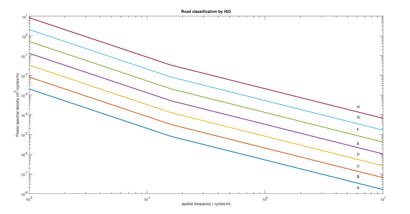
The above plot depicts the ISO road roughness classification from A to H, where class A is determined to be very good, with the least road roughness, and as we go to class H the road roughness increases and the road quality reduces. This standard can be used to determine the quality of road from its PSD data. The plot is the graph between the Power spectral density and the spatial frequency in log scale.

Plot showing the PSD profile

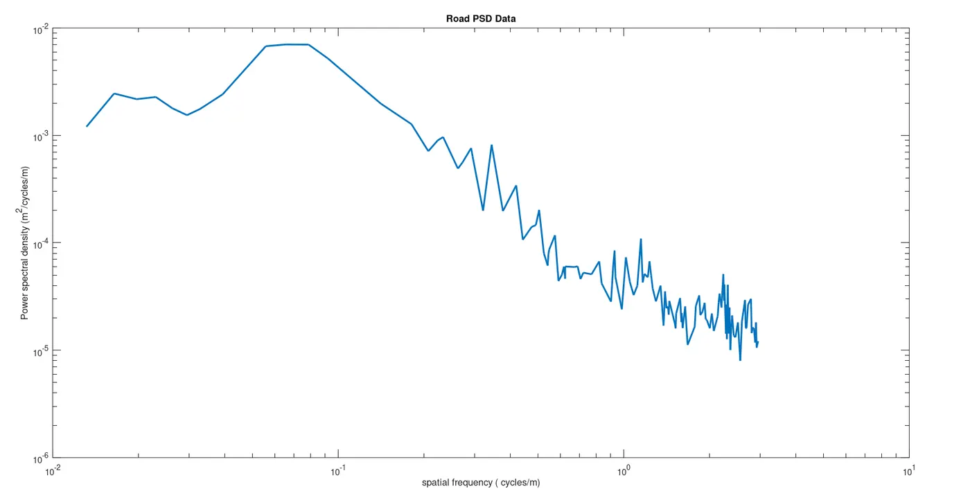
The above plot is the road PSD profile. The road profile is a random signal. So, to analyse it we use the power spectral density to represent it. The PSD profile of road section is unique. Usually all road shows a drop in the amplitude as frequency increase, as it can be infered in the above plot. As the spatial frequency increases, the PSD value reduces. The amplitude is the indication of the road roughness. The magnitude distribution at high and lower spatial frequencies determines the frequency range for less vehicle vibration.

Overlay of PSD profile on ISO classification and determination of road quality

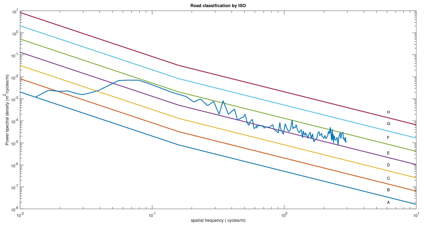
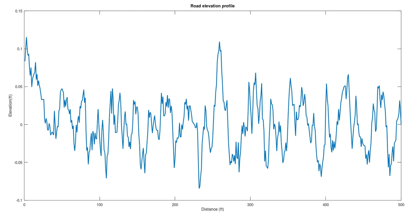
By overlapping the road PSD profile over the ISO standard road roughness class lines, we can determine the rough of the road and thereby infer its quality. In this case, the road data falls in the Class-E band. The degree of roughness for a class E road is given by the range 512*10^-6 to 2048*10^-6 m2/cycles/m. The elevation profile of the road is as follows: