Week 7 - Simulation of a 1D Super-sonic nozzle flow simulation using Macormack Method
OBJECTIVE:
- To solve the conservation and non-conservation form of governing equations of the isentropic flow through a 1D subsonic-supersonic nozzle using the MacCormack method.
- To compute the steady-state temperature distribution of primitive variables and the solutions obtained from the two forms are analyzed.
- To perform a grid independence test on the solutions.
- To compare the normalized mass flow rate distribution between two forms of governing equations
Quasi 1D subsonic-supersonic nozzle flow:
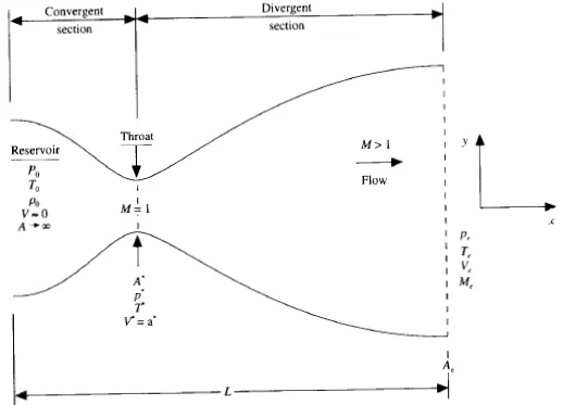
The figure above shows the subsonic-supersonic nozzle. The nozzle consists of three sections: a converging part, a throat section, and a diverging part. The fluid flows through the converging section with a velocity less than that of the speed of sound (Mach number, M < 1), and the flow here is said to be subsonic. The velocity of the fluid at the throat is M = 1 and is transonic. Naturally, since the velocity at the diverging section is greater than the Mach number, one, the section is said to be supersonic.
The flow at the inlet comes from a reservoir which has a large cross-sectional area and hence the area tends to infinity. The resultant velocity tends to zero as well. In the figure, the area of the nozzle changes with respect to the total distance of the nozzle, along x-direction. In reality, the flow properties change along x-y direction but it is assumed that the flow field variables vary along x-direction only (it is equivalent to assuming uniform flow properties across the cross-section) and hence the flow is termed as quasi-1D flow.
Maccormack method:-
The non-dimensionalised governing equations in both conservation and non-conservation form are discretised using Maccormack method. It is a time marching method as in the explicit method but consists of predictor and corrector steps. The equation is forward differenced in the predictor step and the solution is updated using the value obtained. Contrary to the predictor step, in the corrector step, the non_dimensionalised equations are backward differenced and the mean value of time derivative is calculated from both the predictor and corrector values. Finally, the solution for the next time step is calculated using the mean value obtained.
NON-CONSERVATION FORM:-
Continuity equation:

Momentum equation:
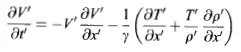
Energy equation:

Boundary conditions at the inlet:


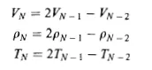
Boundary conditions at the outlet:
Initial Conditions:
Area of the cross-section of the nozzle;

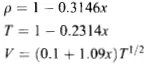
At t=0, the values of the primitive variables be;
CONSERVATION FORM:-
Continuity equation:
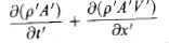
Momentum equation:

Energy equation:

The above three equations in the conservation form cannot be discretised as it is. The primitive variables are initially defined as the elements of the solution vector(U), the flux vector(F) an the source term(J). That is;
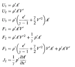
Using the above elements, the non-dimesionalised governing equations in the conservation form can be written as;
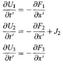
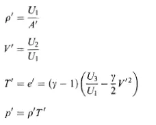
Once the above equations are solved using Maccormack method, the final values of the primitive variables can be determined from the solution vector as:
Boundary condition at the inlet:
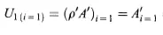

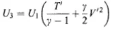
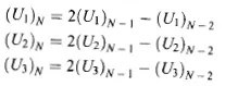
Boundary condition at the outlet:
Initial Conditions:
Area of the cross-section of the nozzle;
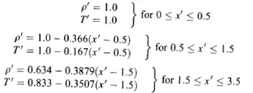
And, the values of the flow-field variables at time, t=0 be;
MAIN CODE:
clear all
close all
clc

%inputs given
L = 3; %length of the nozzle section
n = 31; %number of nodes
x = linspace(0,3,n);
dx = x(2)-x(1);
gamma = 1.4; %ratio of specific heat at constant volume to constant pressure
cfl = 0.5;

%area of the nozzle
a = 1+2.2*(x-1.5).^2;
th = find(a==1);
%number of time steps
nt = 1400;

   %non_conservation form
   m_nc = non_cons_function(x,a,dx,gamma,n,nt,cfl,th);
   m_c = cons_function(x,a,dx,gamma,n,nt,cfl,th);


  figure(7)
  plot(x,m_nc)
  hold on
  plot(x,m_c)
  xlabel('x/L')
  ylabel('mass flow rate')
  title('Steady state massflow rate profiles')
  legend('Non-Conservation','Conservation')
Function For Non-Conservation Form:
%Non-conservation form of governing equations

function m = non_cons_function(x,a,dx,gamma,n,nt,~,th)

%calculating initial profiles
rho = 1-0.3146*x;
t = 1-0.2314*x; % t = temperature
v = (0.1+1.09*x).*t.^0.5;
%mf_rate = rho.*v.*a; %mass flow rate
%p = rho.*t; %pressure ratio
%M = v./sqrt(t); %mach number

%time step_size calculation
% for q = 1:n
% dt_nc(q) = (cfl*dx)./(sqrt(t(q))+v(q));
% end
% dt = min(dt_nc);

dt = 0.0201;
%throat = find(a==1);

%outer time loop
for k = 1:nt
    rho_old = rho;
    v_old = v;
    t_old = t;
    %mf_rate_old = mf_rate;
    %p_old = p;
    %M_old = M;

    %predictor method
    for j = 2:n-1
        dvdx = (v(j+1)-v(j))/dx;
        dlogadx = (log(a(j+1))-log(a(j)))/dx;
        drhodx = (rho(j+1)-rho(j))/dx;
        dtdx = (t(j+1)-t(j))/dx;

        %continuity equation
        drhodt_p(j) = -rho(j)*dvdx-rho(j)*v(j)*dlogadx-v(j)*drhodx;

        %momentum equation
        dvdt_p(j) = -v(j)*dvdx-(1/gamma)*(dtdx+(t(j)/rho(j))*drhodx);

        %energy equation
        dtdt_p(j) = -v(j)*dtdx-(gamma-1)*t(j)*(dvdx+v(j)*dlogadx);

     %solution update
    rho(j) = rho(j)+drhodt_p(j)*dt;
    v(j) = v(j)+dvdt_p(j)*dt;
    t(j) = t(j)+dtdt_p(j)*dt;

    end

%%% Solution update has to be done inside the loop else only the last term will get updated %%%%

    %corrector method
    for j = 2:n-1
        dvdx = (v(j)-v(j-1))/dx;
        dlogadx = (log(a(j))-log(a(j-1)))/dx;
        drhodx = (rho(j)-rho(j-1))/dx;
        dtdx = (t(j)-t(j-1))/dx;

        %continuity equation
        drhodt_corr(j) = -rho(j)*dvdx-rho(j)*v(j)*dlogadx-v(j)*drhodx;

        %momentum equation
        dvdt_corr(j) = -v(j)*dvdx-(1/gamma)*(dtdx+(t(j)/rho(j))*drhodx);

        %energy equation
        dtdt_corr(j) = -v(j)*dtdx-(gamma-1)*t(j)*(dvdx+v(j)*dlogadx);

    end

    %compute the  average time derivative
    drhodt = 0.5*(drhodt_p + drhodt_corr);
    dvdt = 0.5*(dvdt_p + dvdt_corr);
    dtdt = 0.5*(dtdt_p + dtdt_corr);

    %final solution update
    for i = 2:n-1
        rho(i) = rho_old(i)+drhodt(i)*dt;
        v(i) = v_old(i)+dvdt(i)*dt;
        t(i) = t_old(i)+dtdt(i)*dt;
    end

    %apply the boundary conditions
    %at the inlet
    v(1) = 2*v(2)-v(3);
    %t(1) = 1;
    %rho(1) = 1;
    %at the outlet
    v(n) = 2*v(n-1)-v(n-2);
    rho(n) = 2*rho(n-1)-rho(n-2);
    t(n) =2*t(n-1)-t(n-2);

    %computing pressure_ratio, mach_number and mass_flow_rate
    m = rho.*v.*a; %mass flow rate
    p = rho.*t; %pressure ratio
    M = v./sqrt(t); %mach number


    %Values at throat
    rho_th(k) = rho(th);
    M_th(k) = M(th);
    p_th(k) = p(th);
    t_th(k) = t(th);
    v_th(k) = v(th);

    figure(1)
    if k==1
       plot(x,m)
       hold on
    end
    if k==100
       plot(x,m)
       hold on
    end
    if k==200
       plot(x,m)
       hold on
    end
    if k==600
       plot(x,m)
       hold on
    end
    if k==1000
       plot(x,m)
    end

end
xlabel('x')
ylabel('Non-dimensional mass flow')
legend('1dt','100dt','200dt','600dt','1000dt');
title('Instantaneous massflow distribution at six different times')

figure(2)
subplot(4,1,1)
plot(x,rho)
title('Steady state profiles')
xlabel('x')
ylabel('rho')
subplot(4,1,2)
plot(x,v)
xlabel('x')
ylabel('v')
subplot(4,1,3)
plot(x,t)
xlabel('x')
ylabel('t')
subplot(4,1,4)
plot(x,M)
xlabel('x')
ylabel('M')

figure(3)
subplot(4,1,1)
plot(rho_th)
title('Transient state profiles at throat')
%xlabel('x')
ylabel('rho')
subplot(4,1,2)
plot(v_th)
%xlabel('x')
ylabel('v')
subplot(4,1,3)
plot(t_th)
%xlabel('x')
ylabel('t')
subplot(4,1,4)
plot(M_th)
xlabel('Number of time steps')
ylabel('M')


end
Results:
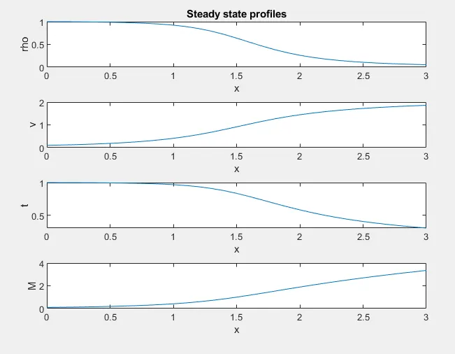
Steady-state distribution of primitive variables inside the nozzle (Fig-1)
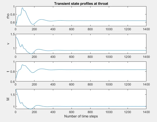
Time-wise variation of primitive variables (Fig-2)
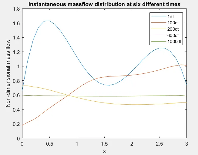
Variation of mass_flow_rate distribution inside the nozzle at different time steps (Fig-3)
Function For Conservation Form:
function m = cons_function(x,a,dx,g,n,nt,~,th)
dt = 0.0267;
for i=1:n
   if x(i)<=0.5
      rho(i) =1;
      t(i) = 1;

   end

      if x(i)>0.5&&x(i)<=1.5
      rho(i) =1-0.366*(x(i)-0.5);
      t(i) = 1-0.167*(x(i)-0.5);
      end

      if x(i)>1.5
      rho(i) =0.634-0.3879*(x(i)-1.5);
      t(i) = 0.833-0.3507*(x(i)-1.5);

   end

end

v = 0.59./(rho.*a);

u1 = rho.*a;
u2 = rho.*a.*v;
u3 = rho.*a.*((t/(g-1))+g*0.5*v.^2);

for k=1:nt
    u1_old = u1;
    u2_old = u2;
    u3_old = u3;

    f1 = u2;
    f2 = u2.^2./u1 + ((g-1)/g)*(u3-0.5*g*u2.^2./u1);
    f3 = g*u2.*u3./u1- 0.5*g*(g-1)*u2.^3./u1.^2;

    for i=2:n-1
     dadx = (a(i+1)-a(i))/dx;
     j2(i)= (1/g)*rho(i)*t(i)*dadx;

     du1dt_p(i) = -(f1(i+1)-f1(i))/dx;
     du2dt_p(i) = -(f2(i+1)-f2(i))/dx + j2(i);
     du3dt_p(i) = -(f3(i+1)-f3(i))/dx;


     u1(i) = u1_old(i) + du1dt_p(i)*dt;
     u2(i) = u2_old(i) + du2dt_p(i)*dt;
     u3(i) = u3_old(i) + du3dt_p(i)*dt;

    end

    f1 = u2;
    f2 = u2.^2./u1 + ((g-1)/g)*(u3-0.5*g*u2.^2./u1);
    f3 = g*u2.*u3./u1- 0.5*g*(g-1)*u2.^3./u1.^2;

    rho = u1./a;
    v = u2./u1;
    t = (g-1)*(u3./u1 - 0.5*g*(u2./u1).^2);

    %Corrector step
     for i=2:n-1
     dadx = (a(i)-a(i-1))/dx;
     j2(i)= (1/g)*rho(i)*t(i)*dadx;

     du1dt_c(i) = -(f1(i)-f1(i-1))/dx;
     du2dt_c(i) = -(f2(i)-f2(i-1))/dx + j2(i);
     du3dt_c(i) = -(f3(i)-f3(i-1))/dx;

     du1dt(i) = 0.5*(du1dt_p(i)+du1dt_c(i));
     du2dt(i) = 0.5*(du2dt_p(i)+du2dt_c(i));
     du3dt(i) = 0.5*(du3dt_p(i)+du3dt_c(i));


     u1(i) = u1_old(i) + du1dt(i)*dt;
     u2(i) = u2_old(i) + du2dt(i)*dt;
     u3(i) = u3_old(i) + du3dt(i)*dt;

    end


    %BC
    %inlet
    u1(1) = a(1);
    u2(1) = 2*u2(2)-u2(3);
    v(1) = u2(1)/u1(1);
    u3(1) = u1(1)*((t(1)/(g-1))+g*0.5*v(1)^2);
    %outlet
    u1(n) = 2*u1(n-1)-u1(n-2);
    u2(n) = 2*u2(n-1)-u2(n-2);
    u3(n) = 2*u3(n-1)-u3(n-2);


    rho = u1./a;
    v = u2./u1;
    t = (g-1)*(u3./u1 - 0.5*g*(u2./u1).^2);
    p = rho.*t;
    M = v./sqrt(t);
    m = rho.*a.*v;

    %Values at throat
    rho_th(k) = rho(th);
    M_th(k) = M(th);
    p_th(k) = p(th);
    t_th(k) = t(th);
    v_th(k) = v(th);

    figure(4)
    if k==1
       plot(x,m)
       hold on
    end
    if k==100
       plot(x,m)
    end
    if k==200
       plot(x,m)
    end
    if k==600
       plot(x,m)
    end
    if k==1000
       plot(x,m)
    end

end
xlabel('x')
ylabel('Non-dimensional mass flow-conservative')
legend('1dt','100dt','200dt','600dt','1000dt');
title('Instantaneous massflow distribution at six different times- Conservative')

figure(5)
subplot(4,1,1)
plot(x,rho)
title('Steady state profiles - Conservative')
xlabel('x')
ylabel('rho')
subplot(4,1,2)
plot(x,v)
xlabel('x')
ylabel('v')
subplot(4,1,3)
plot(x,t)
xlabel('x')
ylabel('t')
subplot(4,1,4)
plot(x,M)
xlabel('x')
ylabel('M')

figure(6)
subplot(4,1,1)
plot(rho_th)
title('Transient state profiles at throat-Conservative')
%xlabel('x')
ylabel('rho')
subplot(4,1,2)
plot(v_th)
%xlabel('x')
ylabel('v')
subplot(4,1,3)
plot(t_th)
%xlabel('x')
ylabel('t')
subplot(4,1,4)
plot(M_th)
xlabel('Number of time steps')
ylabel('M')

end
Results:
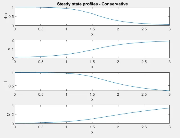
Steady-state distribution of primitive variables inside the nozzle (Fig-4)
Time-wise variation of primitive variables (Fig-5)
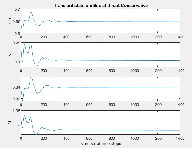
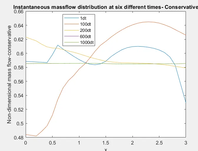
Variation of mass_flow_rate distribution inside the nozzle at different time steps (Fig-6)
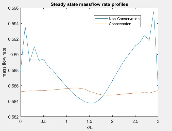
Comparison of normalized mass flow rate distribution of both forms (Fig-7)
INFERENCE:-
- Figures 1 and 4 show the steady-state distribution of the flow variables in the conservation and non-conservation forms. The values of primitive variables are plotted against the non-dimensional nozzle distance after the 1400 time steps. It can be seen that in both forms, the steady-state results are showing the same results with a few noticeable differences.
- Figures 3 and 6 show the transient mass flow plotted against non-dimensional distance across the nozzle for different time step values. It can be seen that the variation in the initial and settled curve in the case of conservation form is much lesser than that of non-conservation form. But this may be due to different initial conditions used in both forms.
- Figure 7 shows the steady-state mass flow variations in conservation and non-conservation forms after 1400 time steps. Here it can be observed that the result obtained from the conservation form is more reliable. The non-conservative figure shows noticeable oscillations at the inlet and outlet. It also shows apparent variation from being a constant in contrast to conservation form. From the Anderson textbook, the analytical solution for mass flow is 0.579, and the conservation form result is closer to that and is satisfactory.
Grid Independence test: When the grid points are changed to 61 from 31, it can be observed that the primitive variables in the conservation form become closer to the analytical solution. Therefore, when grid points are doubled, the steady-state flow-field variable values come closer to that of exact values, indicates the grid-independence of conservation form. But in contrast, with just 31 grid points, the steady-state results of the primitive variables show closer values to the analytical values compared to conservation forms(31/61 grid points).
Conclusion:
- Conservation form conserves mass efficiently and hence the mass flow distribution results are reliable.
- The quality of the numerical algorithm in the case of non-conservation form is better.
- The results obtained for primitive variables in the non-conservation form is more accurate whereas the conservation form yields accurate results for the flux variables.
- Programming is easier in the non-conservation form in comparison to conservation form. This is because more work is needed for conservation form to compute the primitive variables from the flux variables.