Week 5 - Mid term project - Solving the steady and unsteady 2D heat conduction problem
OBJECTIVE: To practice a detailed study on the 2-D heat conduction equation in its steady and transient states by performing different iterative methods.
From the Navier-stokes equation, the 2d heat conduction equation could be derived as:
Transient state:
`(delT)/(delt) = alpha((del^2T)/(delx^2)+(del^2T)/(dely^2))`
Steady-state:
`((del^2T)/(delx^2)+(del^2T)/(dely^2))=0`
Given boundary conditions:
Top boundary temperature, T_T = 600
Bottom boundary temperature, T_B= 900
Left boundary temperature, T_L = 400
Right boundary temperature, T_R =800;
Also, absolute error criteria = 1e-4.
Here, the steady-state solution is solved using the implicit method while the transient-state solution is computed by both explicit and implicit methods. Since the transient state equation contains a time derivative, explicit method can be applied to find the value of the quantity for each time step. This method is time accurate.
In case of implicit methods, we use few iterative techniques to perform the iteration to get the converged solution:
1) Jacobi
2)Gauss-Seidel
3)Successive Over Relaxation (SOR)
Let's denote: T(L) = T(i-1,j)
T(R) = T(i+1,j)
T(T) = T(i,j+1)
T(B) = T(i,j-1)
and,T(P) = T(i,j)
STEADY-STATE ANALYSIS
The steady state equation of the 2d heat equation is descrtized to form:
`T(P)=1/k[((T(L)+T(R))/dx^2)+((T(T)+T(B))/dy^2)]^(n+1)`
where;
`k=(2*(dx^2+dy^2))/(dx^2*dy^2)
Implicit Method:
Matlab code:
%Steady state analysis
%Analytical function
%d2T/dx2 + d2T/sy2 =0

clear all
close all
clc

Lx = 1;
Ly = 1;
nx = 10;
ny = 10;

x = linspace(0,Lx,nx);
dx = x(2)-x(1);
y = linspace(0,Ly,ny);
dy = y(2)-y(1);

error = 9e9;
tol = 1e-4;

%Initialising values
T = 300*ones(nx,ny);
%T_old = T;
%T_initial = T;

%Boundary Conditions
T_T = 600;
T_B= 900;
T_L = 400;
T_R =800;

%Temperature values at the corners
T(1,1) = (T_L+T_T)/2;
T(nx,1)= (T_B+T_L)/2;
T(nx,ny) = (T_R+T_B)/2;
T(1,ny) = (T_R+T_T)/2;

%Assigning boundary values
T(1,2:end-1) = T_T;
T(nx,2:end-1) = T_B;
T(2:end-1,1) = T_L;
T(2:end-1,ny) = T_R;


k = 2*((dx^2+dy^2)/(dx^2*dy^2));
k1 = (1/k)*(1/dx^2);
k2 = (1/k)*(1/dy^2);


iteration_type = input('Enter iteration type:1/2/3 ?')

if(iteration_type==1)
%convergence loop
    jacobi_iteration(T,x,y,nx,ny,tol,k1,k2,error);

elseif iteration_type==2;
%convergence loop
    gauss_iteration(T,x,y,nx,ny,tol,k1,k2,error);

else iteration_type==3;
%convergence loop
    sor_iteration(T,x,y,nx,ny,tol,k1,k2,error);
end- Jacobi: T(J)
`T(P)=1/k[((Told(L)+Told(R))/dx^2)+((Told(T)+Told(B))/dy^2)]`
Function Code for jacobi:
%jacobi iteration method
function jacobi_iteration(T,x,y,nx,ny,tol,k1,k2,error)
jacobi_iter = 1
T_old = T;
while(error>tol) %convergence loop
    for i = 2:nx-1  %space loop
        for j = 2:ny-1
           T(i,j) = k1*T_old(i-1,j)+k1*T_old(i+1,j)+k2*T_old(i,j+1)+k2*T_old(i,j-1);
        end
    end
    error = max(max(abs(T_old - T)));
    T_old = T;
    jacobi_iter = jacobi_iter+1
end

%plotting graph
figure(1)
[X Y]= meshgrid(x,y);
contourf(X,Y,T)
colormap jet
colorbar
xlabel('X')
ylabel('Y')
title_text = sprintf('iteration count= %d',jacobi_iter);
title(title_text)
pause(0.03)
end
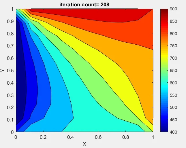
Output figure for jacobi:
- Gauss-Seidel: T(GS)
`T(P)=1/k[((T(L)+Told(R))/dx^2)+((T(T)+Told(B))/dy^2)]`
Function code for gauss-seidel:
%Gauss-Seidel iteration method
function gauss_iteration(T,x,y,nx,ny,tol,k1,k2,error)
gauss_iter = 1
T_old = T;
while(error>tol)%convergence loop
    for i = 2:nx-1 %space loop
        for j = 2:ny-1
           T(i,j) = k1*T(i-1,j)+k1*T_old(i+1,j)+k2*T_old(i,j+1)+k2*T(i,j-1);
        end
    end
    error = max(max(abs(T_old - T)));
    T_old = T;
    gauss_iter = gauss_iter+1
end

%plotting graph
figure(1)
[X Y]= meshgrid(x,y);
contourf(X,Y,T)
colormap jet
colorbar
xlabel('X')
ylabel('Y')
title_text = sprintf('iteration count= %d',gauss_iter);
title(title_text)
pause(0.03)
end
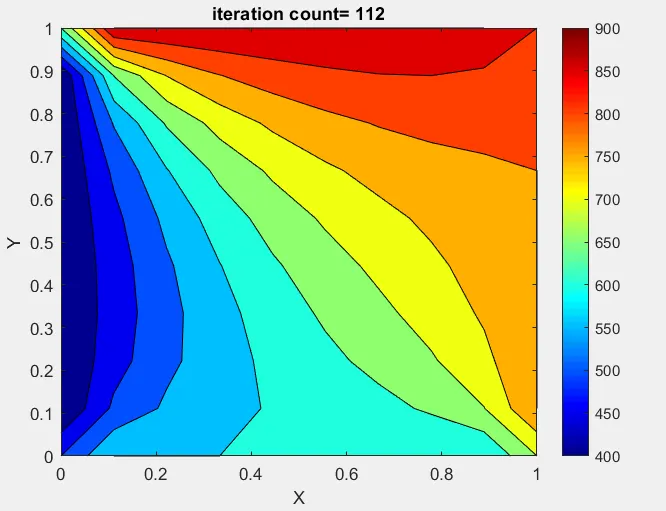
Output graph for gauss-seidel:
- Successive Over Relaxation (SOR)
`T(P)^(k+1) =T(P)^k*(1-alpha)+alpha*(T(GS)orT(J))`
where; alpha is the relaxation factor
Function code for SOR:
%SOR iteration method
function sor_iteration(T,x,y,nx,ny,tol,k1,k2,error)
sor_iter = 1
T_old = T;
alpha = 1.1; %relaxation factor
while(error>tol) %convergence loop
    for i = 2:nx-1 %space loop
        for j = 2:ny-1
           T(i,j) = T_old(i,j)*(1-alpha)+(alpha*(k1*T(i-1,j)+k1*T_old(i+1,j)+k2*T_old(i,j+1)+k2*T(i,j-1)));
        end
    end
    error = max(max(abs(T_old - T)));
    T_old = T;
    sor_iter = sor_iter+1
end

%plotting graph
figure(1)
[X Y]= meshgrid(x,y);
contourf(X,Y,T)
colormap jet
colorbar
xlabel('X')
ylabel('Y')
title_text = sprintf('iteration count= %d',sor_iter);
title(title_text)
pause(0.03)
end
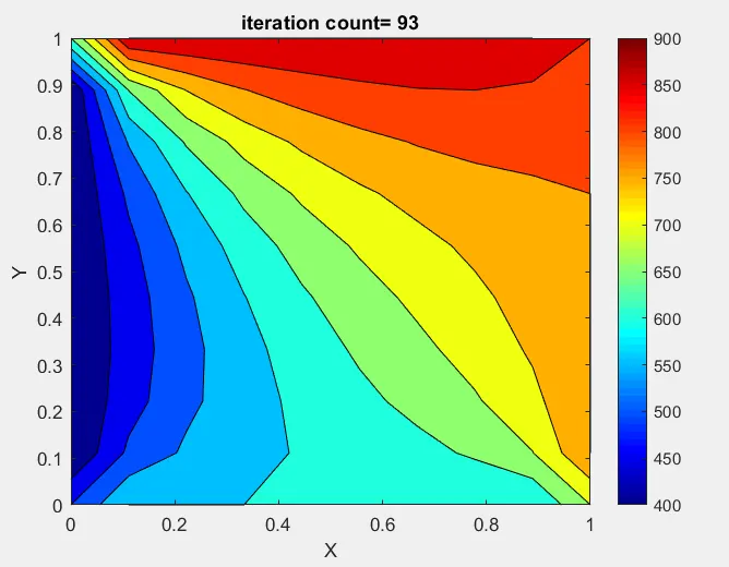
Output graph for SOR:
Observation:
Number of iteration taken for Jacobi =208
Number of iteration taken for gauss-seidel = 112
Number of iteration taken for SOR = 93
It can be seen from here that the SOR method converges the result faster and in a lesser number of iterations.
TRANSIENT-STATE ANALYSIS
Explicit Method:
`T(P)^(n+1)=T(P)^n+alpha*dt((T(R)-2*T(P)+T(L))/dx^2+(T(T)-2*T(P)+T(B))/dy^2)^n`
Matlab code:
%Transient state analysis
%Explicit method
%Analytical function
%dt/dt = alpha*(d2T/dx2 + d2T/sy2)
clear all
close all
clc

Lx = 1;
Ly = 1;
nx = 10;
ny = 10;

x = linspace(0,Lx,nx);
dx = x(2)-x(1);
y = linspace(0,Ly,ny);
dy = y(2)-y(1);

%Initialising values
T = 300*ones(nx,ny);
%Boundary Conditions
T_T = 600;
T_B= 900;
T_L = 400;
T_R =800;

%temperature values at the corners
T(1,1) = (T_L+T_T)/2;
T(nx,1)= (T_B+T_L)/2;
T(nx,ny) = (T_R+T_B)/2;
T(1,ny) = (T_R+T_T)/2;

%assigning temperature at the boundaries
T(1,2:end-1) = T_T;
T(nx,2:end-1) = T_B;
T(2:end-1,1) = T_L;
T(2:end-1,ny) = T_R;

T_old = T;

dt = 30; %time step
nt = 1400;  %assuming number of time steps
alpha = 1.4e-5; %relaxation factor
k1 =(alpha*dt)/dx^2;
k2 = (alpha*dt)/dy^2;

%time loop
loop_counter = 1
for m = 1:nt-1
for i = 2:nx-1 %space loop
    for j = 2:ny-1
        T(i,j)= T_old(i,j)+k1*(T_old(i+1,j)-2*T_old(i,j)+T_old(i-1,j))+k2*(T_old(i,j+1)-2*T_old(i,j)+T_old(i,j-1));

    end

end
%update values
T_old = T;
loop_counter = loop_counter+1
end
[X Y] = meshgrid(x,y);
contourf(X,Y,T)
colormap jet
xlabel('X axis')
ylabel('Y axis')
%set(gca,'YDir','reverse')
%set(gca,'XTick',[],'YTick',[])
colorbar;
%title_text = sprintf('number of iterations = %d',loop_counter)
title('Iteration for time step = 1400')
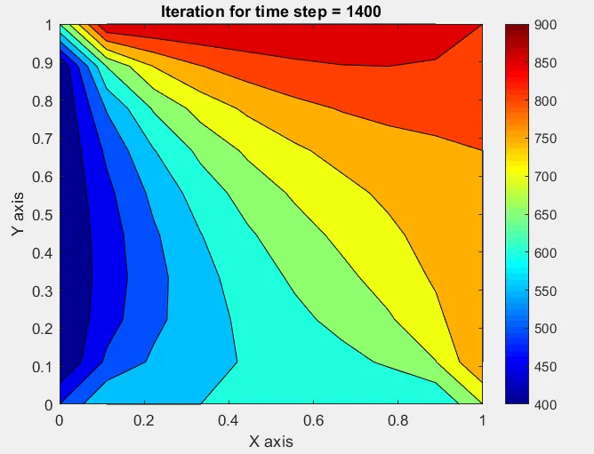
Output graph:
Implicit Method:
`T(P)^(n+1)=(T(P)^n+k1(T(L)^(n+1)+T(R)^(n+1))+k2(T(T)^(n+1)+T(B)^(n+1)))/(1+2*k1+2*k2)`
where;
`k1=(alpha*dt)/dx^2`
`k2=(alpha*dt)/dy^2`
Matlab main code:
%Transient state analysis
%Implicit method
%Analytical function
%dt/dt = alpha*(d2T/dx2 + d2T/sy2)
clear all
close all
clc

Lx = 1;
Ly = 1;
nx = 10;
ny = 10;

x = linspace(0,Lx,nx);
dx = x(2)-x(1);
y = linspace(0,Ly,ny);
dy = y(2)-y(1);

%Initialising values
T = 300*ones(nx,ny);
%Boundary Conditions
T_T = 600;
T_B= 900;
T_L = 400;
T_R =800;

%Temperature at the corners of the grid
T(1,1) = (T_L+T_T)/2;
T(nx,1)= (T_B+T_L)/2;
T(nx,ny) = (T_R+T_B)/2;
T(1,ny) = (T_R+T_T)/2;

%Assigning initial values of the temperatures
T(1,2:end-1) = T_T;
T(nx,2:end-1) = T_B;
T(2:end-1,1) = T_L;
T(2:end-1,ny) = T_R;

error = 9e9;
tol = 1e-4;

dt = 30; %time step
nt = 1400; %number of time steps
alpha = 1.4;
k1 =(alpha*dt)/dx^2;
k2 = (alpha*dt)/dy^2;

method = input('Enter the iteration method:1/2/3?')

if(method==1) %Jacobi
    jacobi_transient(T,x,y,nx,ny,nt,tol,k1,k2,error);
elseif(method==2) %Gauss-siedel
    gauss_transient(T,x,y,nx,ny,nt,tol,k1,k2,error);
else(method==3) %SOR
    sor_transient(T,x,y,nx,ny,nt,tol,k1,k2,alpha,error);
end- Jacobi
`T(P)^(n+1)=(T(P)^n+k1(Told(L)^(n+1)+Told(R)^(n+1))+k2(Told(T)^(n+1)+Told(B)^(n+1)))/(1+2*k1+2*k2)`
Function code for jacobi:
%Transient state
%Implicit method
%method 1
%jacobi iteration method
function jacobi_transient(T,x,y,nx,ny,nt,tol,k1,k2,error)
jacobi_iter = 1
T_prev = T;
T_old = T;
for m = 1:nt  %time loop
    while(error>tol) %convergence loop
    for i = 2:nx-1   %space loop
        for j = 2:ny-1
           term1=(1+(2*k1)+(2*k2))^-1;
           term2=k1*term1;
           term3=k2*term1;
           H=(T_old(i-1,j)+T_old(i+1,j));
           V=(T_old(i,j-1)+T_old(i,j+1));
           T(i,j)=((T_prev(i,j)*term1)+(term2*H)+(term3*V));
        end
    end
    error = max(max(abs(T_old - T)));
    T_old = T;
    jacobi_iter = jacobi_iter+1
    end
T_prev = T;
end
%plotting graph
figure(1)
[X Y]= meshgrid(x,y);
contourf(X,Y,T)
colormap jet
[a b]=contourf(X,Y,T);
clabel(a,b)
xlabel('X')
ylabel('Y')
colorbar
title_text = sprintf('iteration count= %d',jacobi_iter);
title(title_text)
pause(0.03)
end
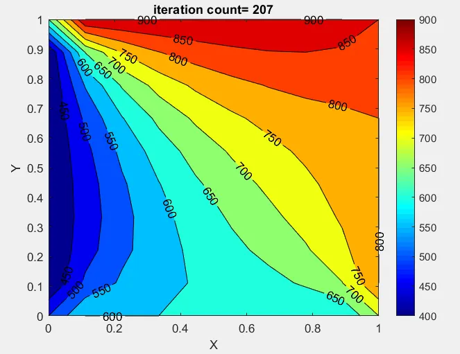
Output graph:
- Gauss-Seidel
`T(P)^(n+1)=(T(P)^n+k1(T(L)^(n+1)+Told(R)^(n+1))+k2(T(T)^(n+1)+Told(B)^(n+1)))/(1+2*k1+2*k2)`
Function code for gauss-seidel:
%Transient state
%Implicit method
%method 1
%jacobi iteration method
function gauss_transient(T,x,y,nx,ny,nt,tol,k1,k2,error)
gauss_iter = 1
T_prev = T;
T_old = T;
for m = 1:nt
    while(error>tol)
    for i = 2:nx-1
        for j = 2:ny-1
           term1=(1+(2*k1)+(2*k2))^-1;
           term2=k1*term1;
           term3=k2*term1;
           H=(T(i-1,j)+T_old(i+1,j));
           V=(T(i,j-1)+T_old(i,j+1));
           T(i,j)=((T_prev(i,j)*term1)+(term2*H)+(term3*V));
        end
    end
    error = max(max(abs(T_old - T)));
    T_old = T;
    gauss_iter = gauss_iter+1
    end
T_prev = T;
end
%plotting graph
figure(1)
[X Y]= meshgrid(x,y);
contourf(X,Y,T)
colormap jet
[a b]=contourf(X,Y,T);
clabel(a,b)
colorbar
xlabel('X')
ylabel('Y')
title_text = sprintf('iteration count= %d',gauss_iter);
title(title_text)
pause(0.03)
end
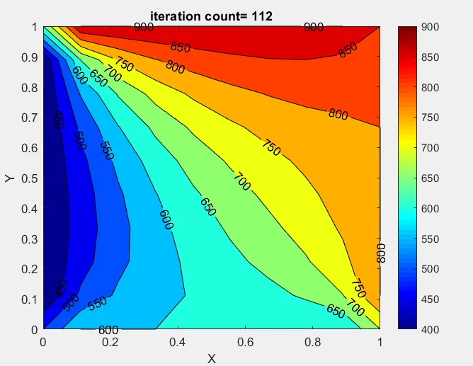
Output graph:
- Successive Over Relaxation (SOR)
`T(P)^(k+1) =T(P)^k*(1-alpha)+alpha*T(GS)`
Function Code for SOR:
%Transient state
%Implicit method
%method 1
%jacobi iteration method
function sor_transient(T,x,y,nx,ny,nt,tol,k1,k2,alpha,error)
sor_iter = 1
T_prev = T;
T_old = T;
for m = 1:nt
    while(error>tol)
    for i = 2:nx-1
        for j = 2:ny-1
           term1=(1+(2*k1)+(2*k2))^-1;
           term2=k1*term1;
           term3=k2*term1;
           H=(T(i-1,j)+T_old(i+1,j));
           V=(T(i,j-1)+T_old(i,j+1));
           T(i,j)=T_old(i,j)*(1-alpha)+(alpha*((T_prev(i,j)*term1)+(term2*H)+(term3*V)));
        end
    end
    error = max(max(abs(T_old - T)));
    T_old = T;
    sor_iter = sor_iter+1
    end
T_prev = T;
end
%plotting graph
figure(1)
[X Y]= meshgrid(x,y);
contourf(X,Y,T)
colormap jet
[a b]=contourf(X,Y,T);
clabel(a,b)
colorbar
xlabel('X')
ylabel('Y')
title_text = sprintf('iteration count= %d',sor_iter);
title(title_text)
pause(0.03)
end
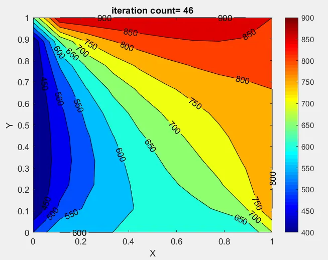
Output graph:
Observation:
Number of iterations in Jacobi = 207
Number of iterations in gauss-seidel = 112
Number of iterations in SOR = 467
Hence, successive over-relaxation method yields faster convergence of the solution as compared to the other two methods. SOR is therefore more efficient and can be used for lesser computation time.