Week 3 - Taylor table method and Matlab code

Objective: to derive a fourth-order approximation of second-order derivative for central difference, skewed right-sided, and left-sided methods. Also, to verify the derived right-sided and left-sided skewed schemes are fourth-order accurate.

Initially, let's assume a hypothesis function for the analytical function, and the number of terms in the hypothesis function is determined from the hint given for each scheme. Let P be the order of approximation, Q be the order of derivative, and N be the number of nodes in the numerical stencil.

Hence, for central differencing, N = P+Q-1 & for skewed difference, N = P+Q. Since we are solving for second-order derivative using fourth-order approximation, P = 4 and Q =2

We are using the Taylor table method here to do the derivation. Essentially, we arrange the number of terms from the hypothesis function and the associated Taylor series in the Taylor table.

Central Difference :

Let the number of nodes, N = 4+2-1=5

Therefore, hypothesis function be : `(DeltaX^2)(del^2f)/(delx^2) = a.f(i-2)+b.f(i-1)+c.f(i)+d.f(i+1)+e.f(i+2)`

whereas; i is the position of the node

The values of a, b, c, d and e will be determined from the Taylor table.

Taylor table:-

`(del^2f)/(delx^2)`	`f(x)`	`f'(x) dx`	`f''(dx)^2`	`f'''(x)(dx)^3`	`f^(IV) (dx)^4`	`f^V (dx)^5`	`f^(VI)(dx)^6`
a.f(i-2)	a	-2a	2a	-4a/3	2a/3	-4a/15	4a/45
b.f(i-1)	b	-b	b/2	-b/6	b/24	-b/120	b/720
c.f(i)	c	0	0	0	0	0	0
d.f(i+1)	d	d	d/2	d/6	d/24	d/120	d/720
e.f(i+2)	e	2e	2e	4e/3	2e/3	4e/15	4e/45
Sum	0	0	1	0	0	?	?

On comparing and equating the coefficients of different orders of derivatives in the Taylor series with the function, we get from the table a few equations with respective unknowns. They are;

a+b+c+d+e = 0

-2a-b+d+2e = 0

2a+(b/2)+(d/2)+2e = 1

(-4a/3)-(b/6)+(d/6)+(4e/3) = 0

(2a/3)+(b/24)+(d/24)+(2e/3) = 0

Let's solve the above coupled equations using Matrix Inversion Method.

`A = [[1,1,1,1,1],[-2,-1,0,1,2],[2,1/2,0,1/2,2],[-4/3,-1/6,0,1/6,4/3],[2/3,1/24,0,1/24,2/3]]`

`X = [[a],[b],[c],[d],[e]]`

`B = [[0],[0],[1],[0],[0]]`

By matrix inversion method, `X=A^-1B`

Hence, `[[a],[b],[c],[d],[e]] = [[-0.0833],[1.3333],[-2.5],[1.3333],[-0.0833]]`

We can observe from the solution that a=e and b=d.

Hence, `(del^2f)/(delx^2) = (-0.0833f(i-2)+1.3333f(i-1)-2.5f(i)+1.3333f(i+1)-0.0833f(i+2))/(DeltaX^2)`

Skewed right-sided difference:

Number of nodes assumed, N = 4+2 = 5

Hence the hypothesis equation be : `(DeltaX^2)(del^2f)/(delx^2) = a.f(i)+b.f(i+1)+c.f(i+2)+d.f(i+3)+e.f(i+4)+g.f(i+5)`

`(del^2f)/(delx^2)`	`f(x)`	`f'(x) dx`	`f''(x)(dx)^2`	`f'''(x)(dx)^3`	`f^(IV)(x) (dx)^4`	`f^V(x) (dx)^5`	`f^(VI)(x)(dx)^6`
a.f(i)	a	0	0	0	0	0	0
b.f(i+1)	b	b	b/2	b/6	b/24	b/120	b/720
c.f(i+2)	c	2c	4c/2	8c/6	16c/24	32c/120	4c/45
d.f(i+3)	d	3d	9d/2	27d/6	81d/24	243d/120	81d/80
e.f(i+4)	e	4e	16e/2	64e/6	256e/24	1024e/120	256e/45
f.f(i+5)	g	5g	25g/2	125g/6	625g/24	3125g/120	3125 g/144
Sum	0	0	1	0	0	0	?

From the Taylor table above, we come up with 6 coupled polynomials with 6 unknowns a, b, c, d, e, and g.

a+b+c+d+e+g = 0

b+2c+3d+4e+5g = 0

(b/2)+(4c/2)+(9d/2)+(16e/2)+(25g/2) = 1

(b/6)+(8c/6)+(27d/6)+(64e/6)+(125g/6) = 0

(b/24)+(16c/24)+(81d/24)+(256e/24)+(625g/24) = 0

(b/120)+(32c/120)+(243d/120)+(1024e/120)+(3125g/120) = 0

`A = [[1,1,1,1,1,1],[0,1,2,3,4,5],[0,1/2,4/2,9/2,16/2,25/2],[0,1/6,8/6,27/6,64/6,125/6],[0,1/24,16/24,81/24,256/24,625/24],[0,1/120,32/120,243/120,1024/120,3125/120]]`

`X = [[a],[b],[c],[d],[e],[g]]`

`B = [[0],[0],[1],[0],[0],[0]]`

Solving for X to find the values of coefficients using matrix inversion method:

`[[a],[b],[c],[d],[e],[g]] = [[3.75],[-12.8333],[17.8333],[-13],[5.0833],[-0.8333]]`

Therefore the 4th order skewed right-sided difference approximation for the 2nd order derivative is:

`(del^2f)/(delx^2) = (3.75f(i)-12.8333f(i+1)+17.8333f(i+2)-13f(i+3)+5.0833f(i+4)-0.8333f(i+5))/(DeltaX^2)`

Proof of 4th order accuracy:

Substituing the values of a, b, c, d, e and g in the equation of Taylor series of second order derivative, we get:

`(del^2f)/(delx^2) = [(-12.8333/2)+((4*17.8333)/2)+((9*-13)/2)+((16*5.0833)/2)+((25*-0.8333))/2]*f''(x)*(dx)^2+ [(-12.8333/120)+((4*17.8333))/45+((81*-13))/80+((256*5.0833)/45)+((3125*-0.8333)/144)]*f^(VI)(x)*(dx)^6`

`implies a.f(i)+b.f(i+1)+c.f(i+2)+d.f(i+3)+e.f(i+4)+g.f(i+5) = f''(x)*(dx)^2 + (-0.8497)*f^(VI)*(dx)^6`

Dividing both LHS and RHS by dx^2 we get:

`(a.f(i)+b.f(i+1)+c.f(i+2)+d.f(i+3)+e.f(i+4)+g.f(i+5))/dx^2 = f''(x)+ (-0.8497)*f^(VI)*(dx)^4`

Since the term that we truncate consists of dx with a degree of 4, it is confirmed that skewed right-sided is fourth order accurate.

Skewed left-sided difference:

Number of nodes assumed, N = 4+2 = 5

Hence the hypothesis equation be : `(DeltaX^2)(del^2f)/(delx^2) = a.f(i-5)+b.f(i-4)+c.f(i-3)+d.f(i-2)+e.f(i-1)+g.f(i)`

`(del^2f)/(delx^2)`	`f(x)`	`f'(x) dx`	`f''(dx)^2`	`f'''(x)(dx)^3`	`f^(IV) (dx)^4`	`f^V (dx)^5`	`f^(VI)(dx)^6`
a.f(i-5)	a	-5a	25a/2	-125a/6	625a/24	-3125a/120	3125 a/144
b.f(i-4)	b	-4b	16b/2	-64b/6	256b/24	-1024b/120	256b/45
c.f(i-3)	c	-3c	9c/2	-27c/6	81c/24	-243c/120	81c/80
d.f(i-2)	d	-2d	4d/2	-8d/6	16d/24	-32d/120	4d/45
e.f(i-1)	e	-e	e/2	-e/6	e/24	-e/120	e/720
f.f(i)	g	0	0	0	0	0	0
Sum	0	0	1	0	0	0	?

From the Taylor table above, we come up with 6 coupled polynomials with 6 unknowns a, b, c, d, e, and g.

a+b+c+d+e+g = 0

-5a-4b-3c-2d-e = 0

(25a/2)+(16b/2)+(9c/2)+(4d/2)+(e/2) = 1

(-125a/6)+(-64b/6)+(-27c/6)+(-8d/6)+(-e/6) = 0

(625a/24)+(256b/24)+(81c/24)+(16d/24)+(e/24) = 0

(-3125a/120)+(-1024b/120)+(-243c/120)+(-32d/120)+(-e/120) = 0

Let's solve the above coupled equations using Matrix Inversion Method.

`A = [[1,1,1,1,1,1],[-5,-4,-3,-2,-1,0],[25/2,16/2,9/2,4/2,1/2,0],[-125/6,-64/6,-27/6,-8/6,-1/6,0],[625/24,256/24,81/24,16/24,1/24,0],[-3125/120,-1024/120,-243/120,-32/120,-1/120,0]]`

`B = [[0],[0],[1],[0],[0],[0]]`

`X = [[a],[b],[c],[d],[e],[g]]`

Solving for X to find the values of coefficients using matrix inversion method:

`[[a],[b],[c],[d],[e],[g]] = [[-0.8333],[5.0833],[-13],[17],[-12.8333],[3.75]]`

Hence, 4th order approximation of the skewed left-sided difference for the 2nd order derivative is:

`(del^2f)/(delx^2) = (3.75f(i)-12.8333f(i+1)+17.8333f(i+2)-13f(i+3)+5.0833f(i+4)-0.8333f(i+5))/(DeltaX^2)`

Proof of 4th order accuracy:

Substituing the values of coefficients determined in the equation of Taylor series, we get:

`(del^2f)/(delx^2) = [(25*-0.8333)/2)+((16*5.0833))/2+((9*-13))/2+((4*17)/2)+((3.75)/2)]*f''(x)dx^2+[(3125*-0.8333)/144)+((256*5.0833)/45)+((81*-13)/80)+((4*17)/45)+((3.75))/720]*f^(VI)(x)*(dx)^6`

`implies (del^2f)/(delx^2) = f''(x)dx^2+[-0.8353]*f^(VI)(x)*(dx)^6`

`(a.f(i-5)+b.f(i-4)+c.f(i-3)+d.f(i-2)+e.f(i-1)+g.f(i))/dx^2 = f''(x)+ (-0.8353)*f^(VI)*(dx)^4`

Since in the above equation, we are truncating a term with a degree of 4 with respect to dx, it is proved that skewed left-sided approximation is 4th order accurate.

Main Matlab code used:

%computing 2nd order derivative 
%using central, skewed right-sided and left-sided schemes
%analytical function = exp(x)*cos(x)

clear all
close all
clc
%let's asssume inputs
x = pi/3;
dx = linspace(pi/4,pi/400,40);

%analytical derivative
%second order derivative
%analytical_derivative = -2*exp(x)*sin(x)

for i = 1:length(dx)
    central_difference_error(i)= central_difference_approx(x,dx(i));
    skewed_rightsided_error(i)= skewed_right_approx(x,dx(i));
    skewed_leftsided_error(i)=skewed_left_approx(x,dx(i));
end

%plotting graph
%comparing central, skewed right-sided and left-sided
figure(1)
loglog(dx,central_difference_error,'-bs')
hold on
loglog(dx,skewed_rightsided_error,'-blacks')
hold on
loglog(dx,skewed_leftsided_error,'-ro')
xlabel('grid size(dx)')
ylabel('Absolute Error')
legend('Central difference scheme','Skewed right-sided scheme','Skewed left-sided scheme')

Function code: Central Difference

function central_out = central_difference_approx(x,dx)
%analytical function = exp(x)*cos(x);
%analytical second order derivative
analytical_derivative = -2*exp(x)*sin(x);

%numerical derivative
a = -1/12;
b = 16/12;
c = -30/12;
d = 16/12;
e = -1/12;

f1 = exp(x-2*dx)*cos(x-2*dx);
f2 = exp(x-dx)*cos(x-dx);
f3 = exp(x)*cos(x);
f4 = exp(x+dx)*cos(x+dx);
f5 = exp(x+2*dx)*cos(x+2*dx);
%central_difference = (a*exp(x-2*dx)*cos(x-2*dx)+b*exp(x-dx)*cos(x-dx)+c*exp(x)*cos(x)+d*exp(x+dx)*cos(x+dx)+e*exp(x+2*dx)*cos(x+2*dx))/(dx)^2;
central_difference = (a*f1+b*f2+c*f3+d*f4+e*f5)/dx^2;
central_out = abs(analytical_derivative-central_difference);
end

Function Code: Skewed Right-Sided Difference

function right_out = skewed_right_approx(x,dx)
%analytical function = exp(x)*cos(x);
%analytical second order derivative
analytical_derivative = -2*exp(x)*sin(x);

%numerical derivative
a = 45/12;
b = -154/12;
c = 214/12;
d = -156/12;
e = 61/12;
g = -10/12;

f1 = exp(x)*cos(x);
f2 = exp(x+dx)*cos(x+dx);
f3 = exp(x+(2*dx))*cos(x+(2*dx));
f4 = exp(x+(3*dx))*cos(x+(3*dx));
f5 = exp(x+(4*dx))*cos(x+(4*dx));
f6 = exp(x+(5*dx))*cos(x+(5*dx));

right_sided_difference = (a*f1+b*f2+c*f3+d*f4+e*f5+g*f6)/dx^2;
%right_sided_difference = ((a*(exp(x)*cos(x)))+(b*(exp(x+dx)*cos(x+dx)))+(c*(exp(x+(2*dx))*cos(x+(2*dx))))+(d*(exp(x+(3*dx))*cos(x+(3*dx))))+(e*(exp(x+(4*dx))*cos(x+(4*dx))))+(g*(exp(x+(5*dx))*cos(x+(5*dx)))))/(dx)^2;
right_out = abs(analytical_derivative-right_sided_difference);
end

Function Code: Skewed Left-Sided Difference

function left_out = skewed_left_approx(x,dx)
%analytical function = exp(x)*cos(x);
%analytical second order derivative
analytical_derivative = -2*exp(x)*sin(x);

%numerical derivative
a = -10/12;
b = 61/12;
c = -156/12;
d = 214/12;
e = -154/12;
g = 45/12;

f1 = exp(x-5*dx)*cos(x-5*dx);
f2 = exp(x-4*dx)*cos(x-4*dx);
f3 = exp(x-3*dx)*cos(x-3*dx);
f4 = exp(x-2*dx)*cos(x-2*dx);
f5 = exp(x-dx)*cos(x-dx);
f6 = exp(x)*cos(x);

left_sided_difference = (a*f1+b*f2+c*f3+d*f4+e*f5+g*f6)/dx^2
%left_sided_difference = ((a*(exp(x-(5*dx))*cos(x-(5*dx))))+(b*(exp(x-(4*dx))*cos(x+(4*dx))))+(c*(exp(x-(3*dx))*cos(x+(3*dx))))+(d*(exp(x+(2*dx))*cos(x+(2*dx))))+(e*(exp(x+dx)*cos(x+dx)))+(g*(exp(x)*cos(x))))/(dx)^2;
left_out = abs(analytical_derivative-left_sided_difference);
end

Output graph: Comparison of absolute errors of central/Skewed(right-sided & left-sided) with respect to grid size.

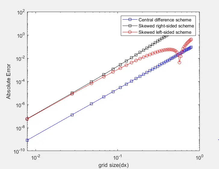
It can be clearly seen from the graph above that the rate at which the error converges in case of central difference is more than that of the rest of the schemes. Hence, when comparing the central difference method with the other two methods, we can say that it's more reliable since the error is minimal.

But when we have to compute the values of the function at the boundaries of the domain, we can not depend on the central difference method as we can not use the nodes on either side of the nodes of interest. In this scenario, depending on the direction of the flow of information, we can use either skewed right-sided or skewed left-sided schemes. Although initially, the skewed left-sided method shows little error than the right-sided counterpart, when grid size becomes finer, both seem to be converging.

Also, the round-off error seems to play a major role in building error. Hence, in higher degree approximations, it is always advised to use coefficients in the fractional form to avoid round-off errors. In addition to that, it is seen that round-off error is introduced when grid size gets finer and desired output may not be obtained.