Week 1- Mixing Tee

STUDY AND ANALYSIS OF MIXING EFFECTIVENESS INSIDE A MIXING TEE

OBJECTIVE:

• The steady-state simulations of the mixing tee are to be performed for two cases with different parameters.
• The effectiveness of the mixing inside the geometries with different parameters is compared and analyzed.

Given:

Hot inlet temperature = 36°C

Cold inlet temperature = 19°C

Hot inlet velocity for the short/long mixing tee = 3 m/s

Momentum ratios = 2 and 4 taken for each case

Momentum Ratio (MR) = (Velocity at the cold inlet) /(Velocity at the hot inlet)

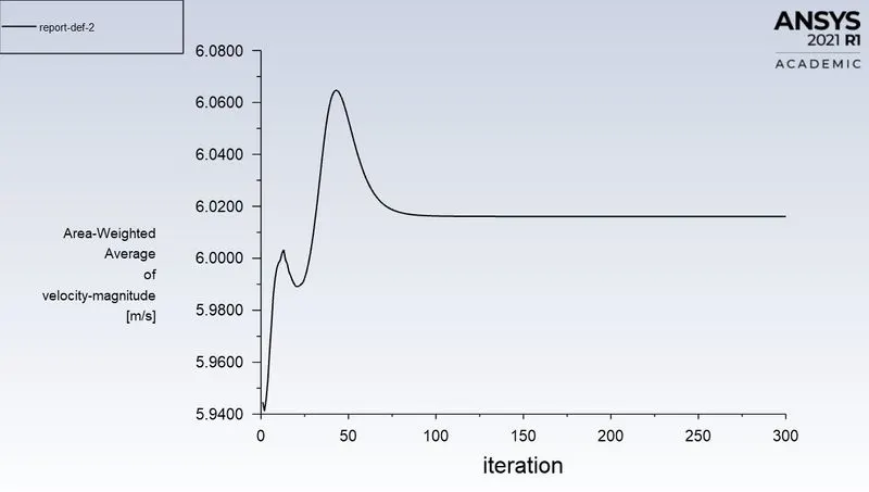
Therefore, when MR is 2, the velocity at the cold inlet is 6 m/s and the same is 12 m/s when MR is 4.

Baseline Mesh (using k-epsilon and default mesh size)

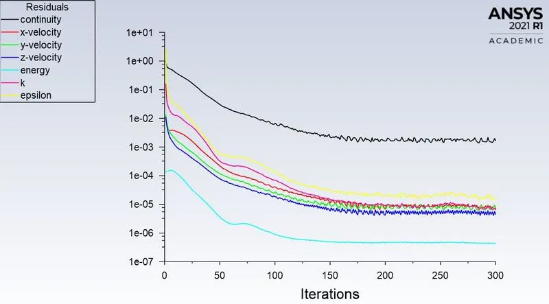
Convergence Plot:

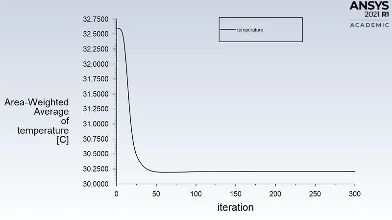
Temperature Plot:

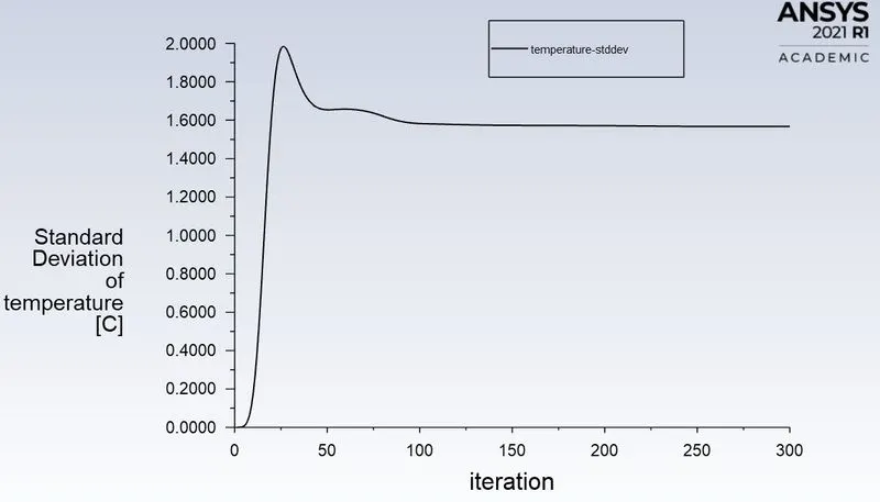
Standard Deviationtion for Temperature:

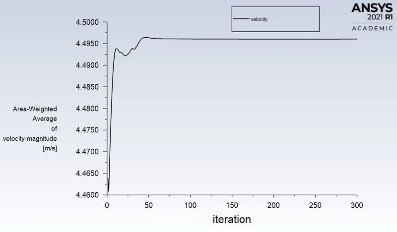
Velocity Plot:

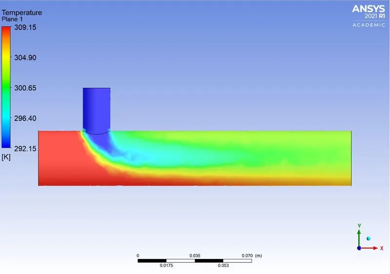
Contour Plot for Temperature (along the length of fluid flow):

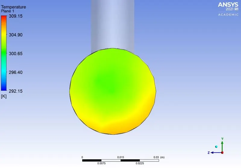
Contour Plot for Temperature (across the length of fluid flow):

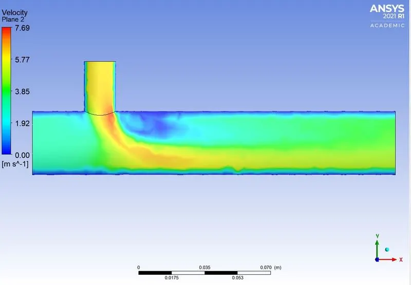
Contour Plot for Velocity (along the length of fluid flow):

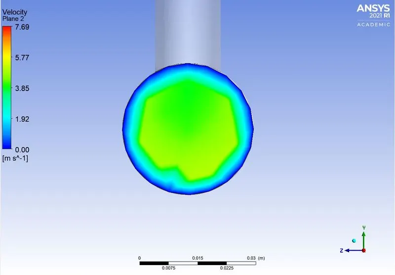
Contour Plot for Velocity (across the length of fluid flow):

Baseline Mesh (using k-omega and default mesh size)

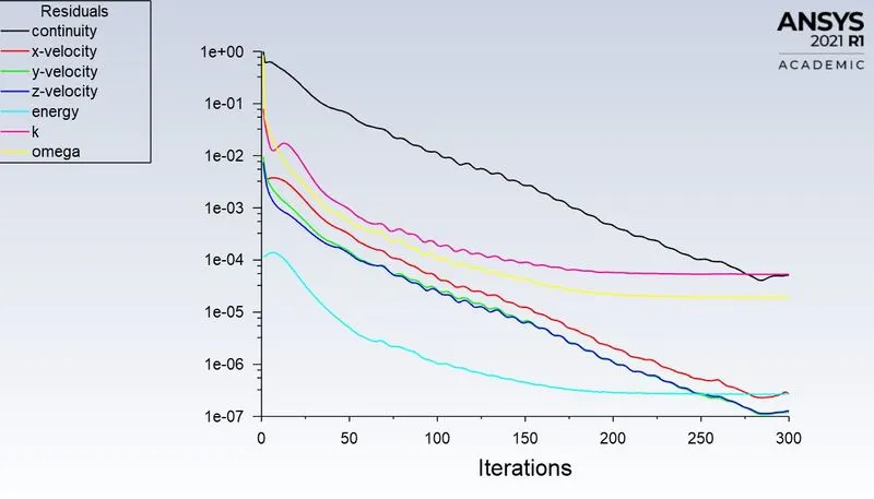
Convergence Plot:

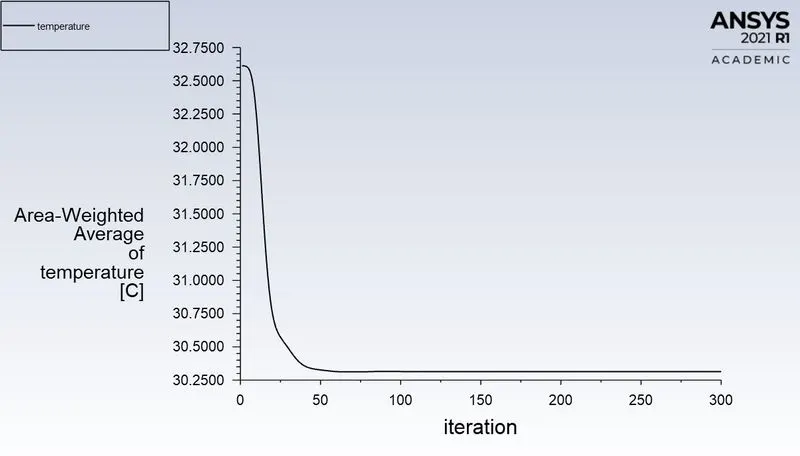
Temperature Plot:

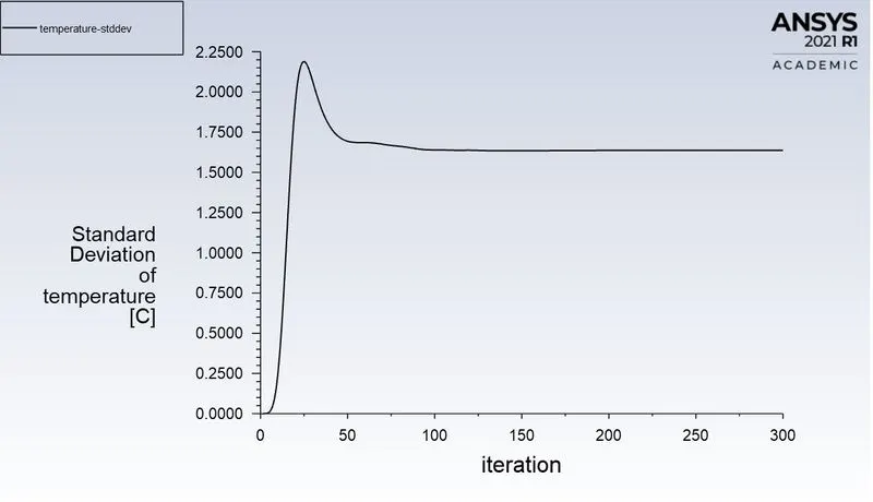
Standard Deviationtion for Temperature:

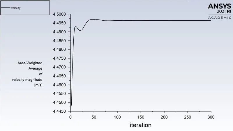
Velocity Plot:

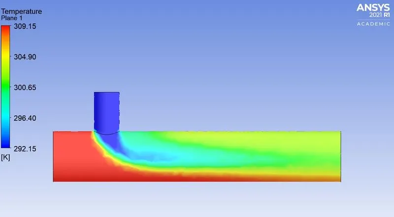
Contour Plot for Temperature (along the length of fluid flow):

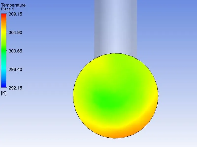
Contour Plot for Temperature (across the length of fluid flow):

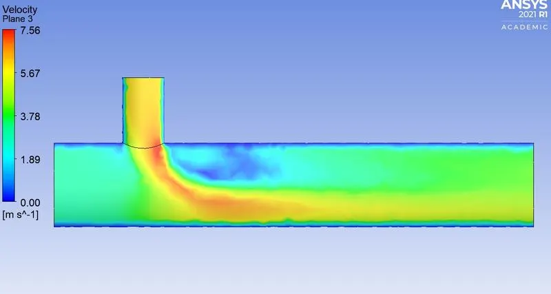
Contour Plot for Velocity (along the length of fluid flow):

Contour Plot for Velocity (across the length of fluid flow):

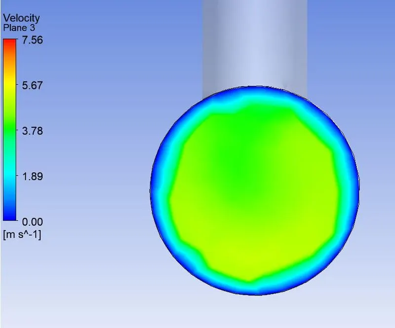
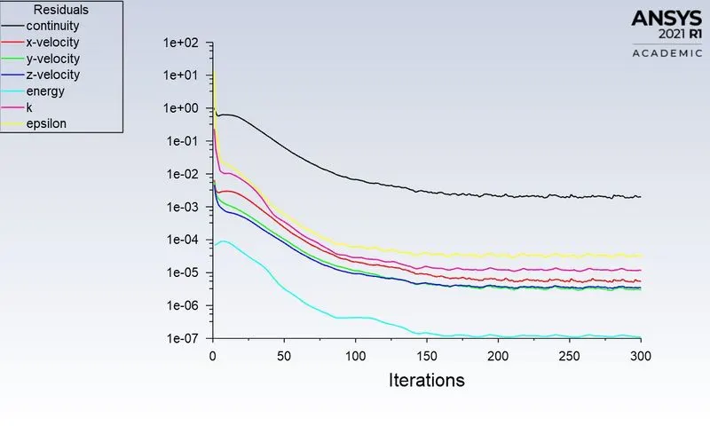
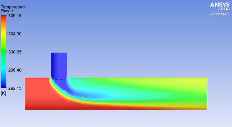
Here the baseline mesh is simulated using both k-epsilon and k-omega models and it is found that simulation using the k-epsilon model is decently converging while K-omega is not. Therefore, it can be interpreted that the k-epsilon works well away from the wall predictions while the k-omega model is for near-wall predictions.

CASE 1: Short mixing tee

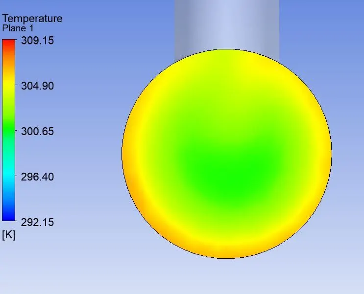
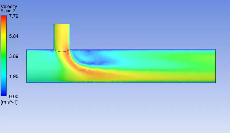
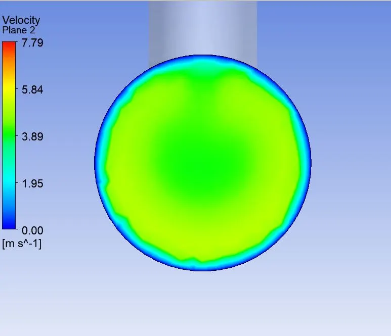
• When hot inlet velocity = 3 m/s and momentum ratio =2

Convergence Plot:

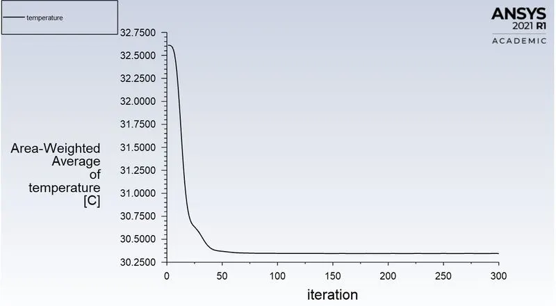
Temperature Plot:

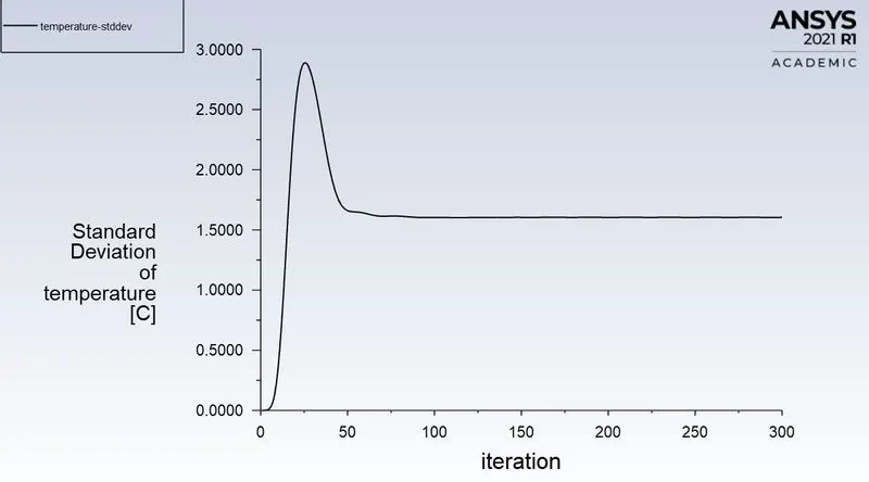
Standard Deviationtion for Temperature:

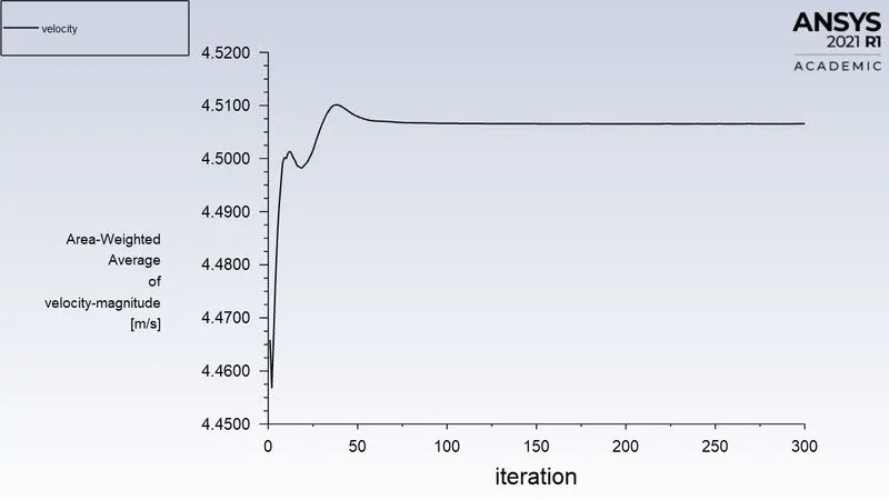
Velocity Plot:

Contour Plot for Temperature (along the length of fluid flow):

Contour Plot for Temperature (across the length of fluid flow):

Contour Plot for Velocity (along the length of fluid flow):

Contour Plot for Velocity (across the length of fluid flow):

• When hot inlet velocity = 3 m/s and momentum ratio =4

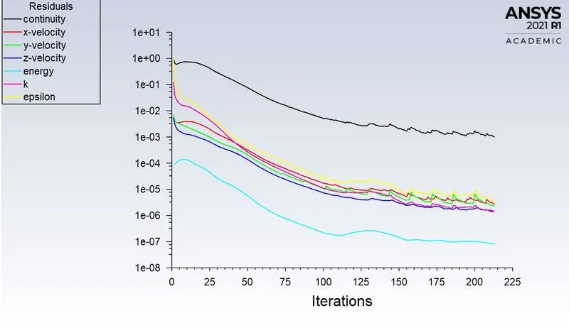
Convergence Plot:

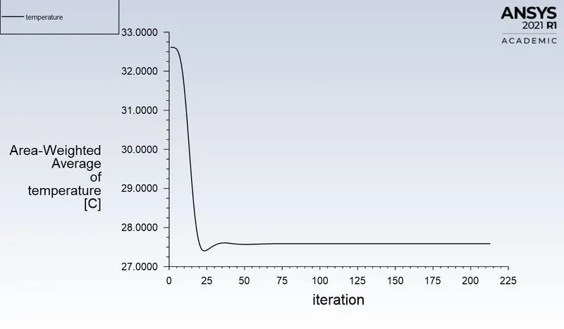
Temperature Plot:

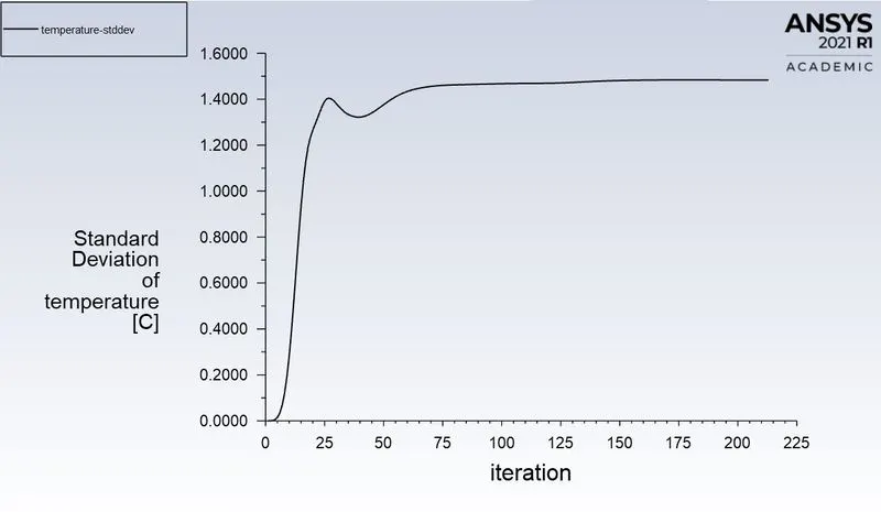
Standard Deviationtion for Temperature:

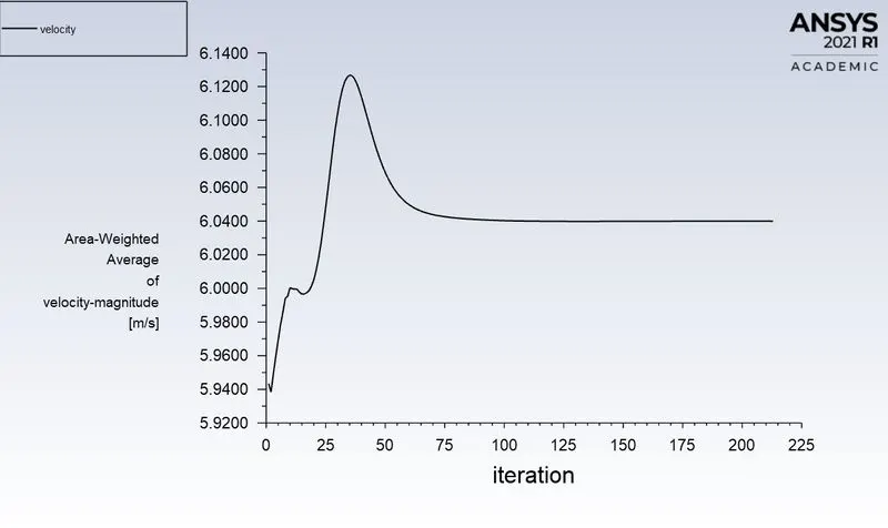
Velocity Plot:

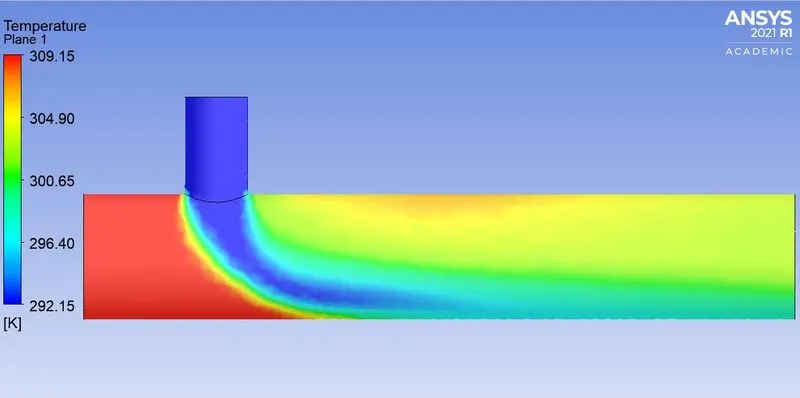
Contour Plot for Temperature (along the length of fluid flow):

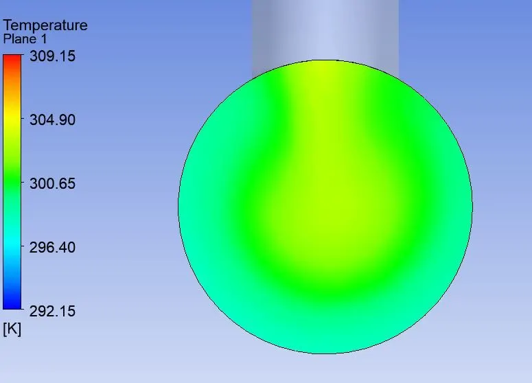
Contour Plot for Temperature (across the length of fluid flow):

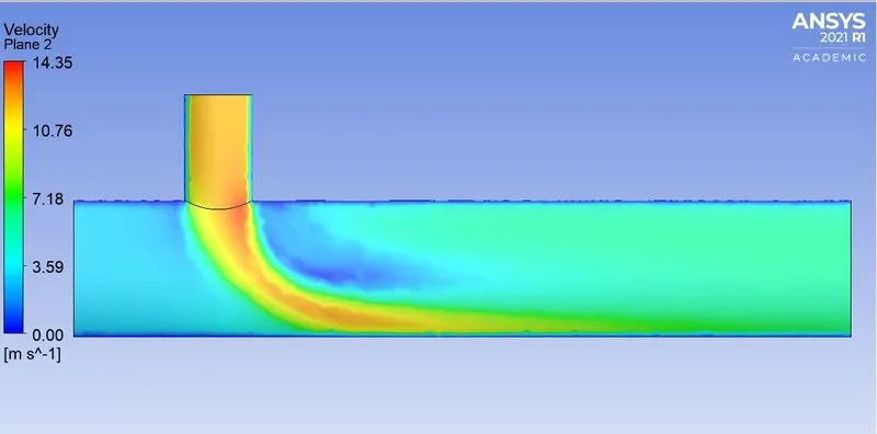
Contour Plot for Velocity (along the length of fluid flow):

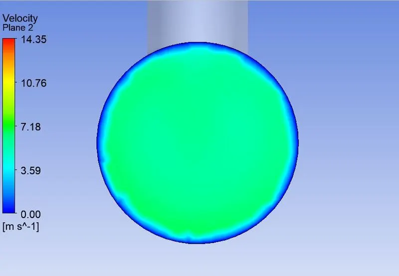
Contour Plot for Velocity (across the length of fluid flow):

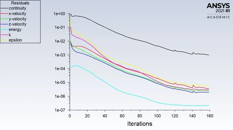
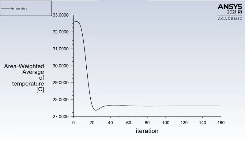
Short mixing tee with mesh grid size 3 mm

Convergence Plot

Temperature Plot

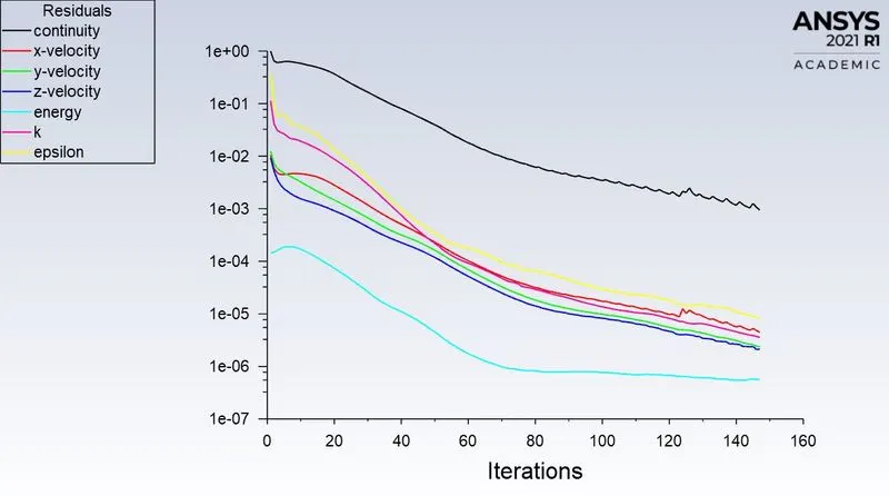
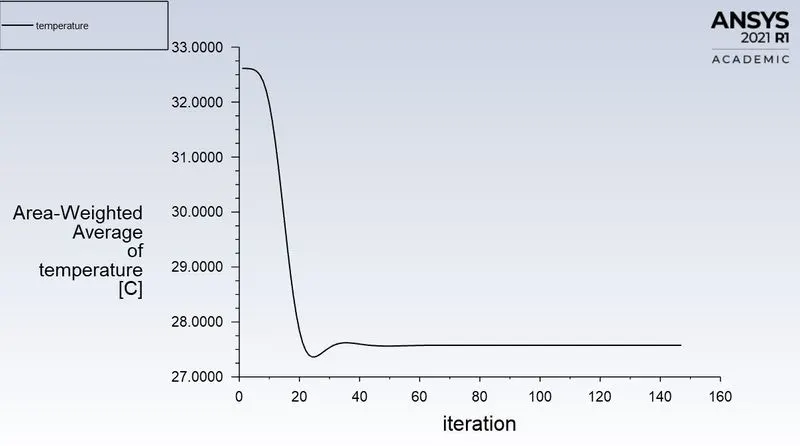
Short mixing tee with mesh grid size 4 mm

Convergence Plot

Temperature Plot

CASE 2: Long mixing tee

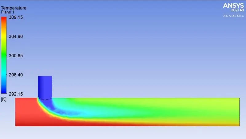
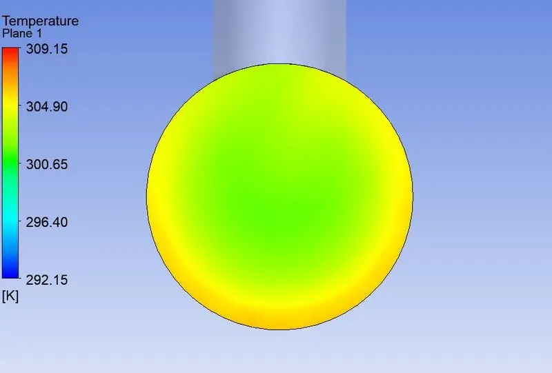
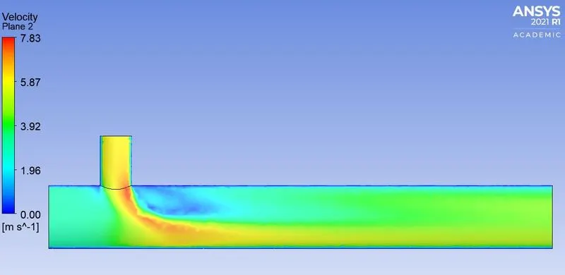
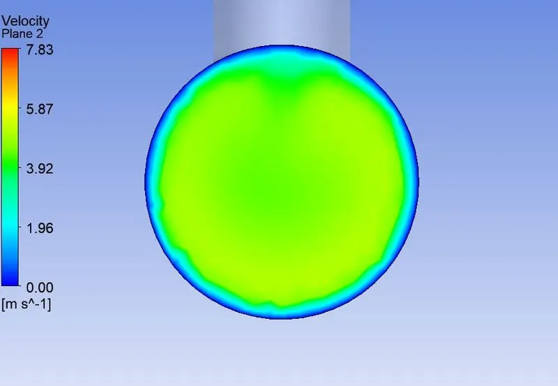
• When hot inlet velocity = 3 m/s and momentum ratio =2

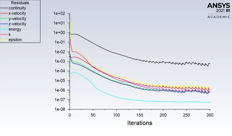
Convergence Plot:

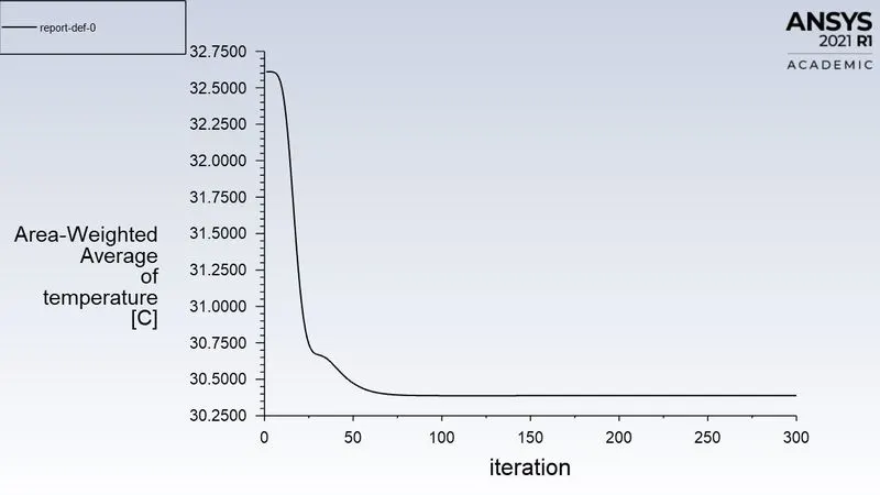
Temperature Plot:

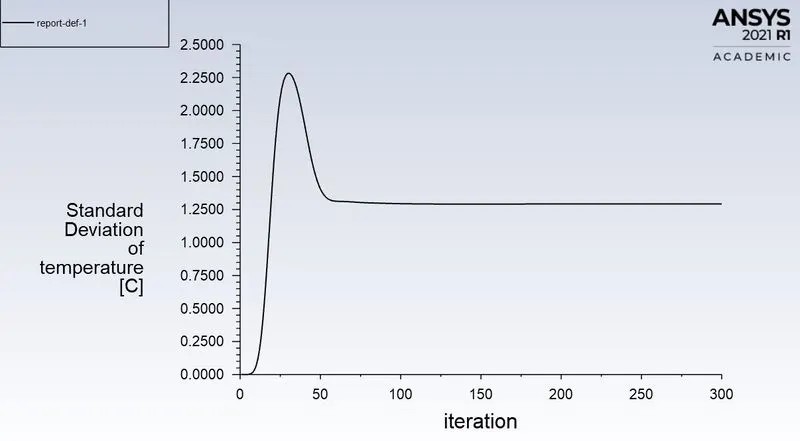
Standard Deviationtion for Temperature:

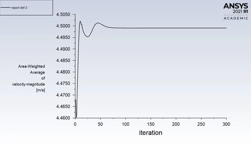
Velocity Plot:

Contour Plot for Temperature (along the length of fluid flow):

Contour Plot for Temperature (across the length of fluid flow):

Contour Plot for Velocity (along the length of fluid flow):

Contour Plot for Velocity (across the length of fluid flow):

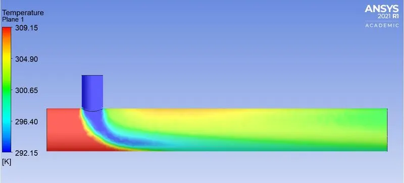
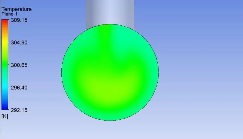
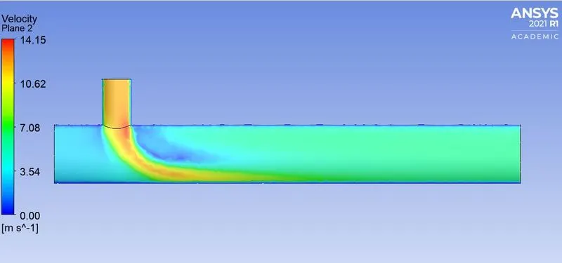
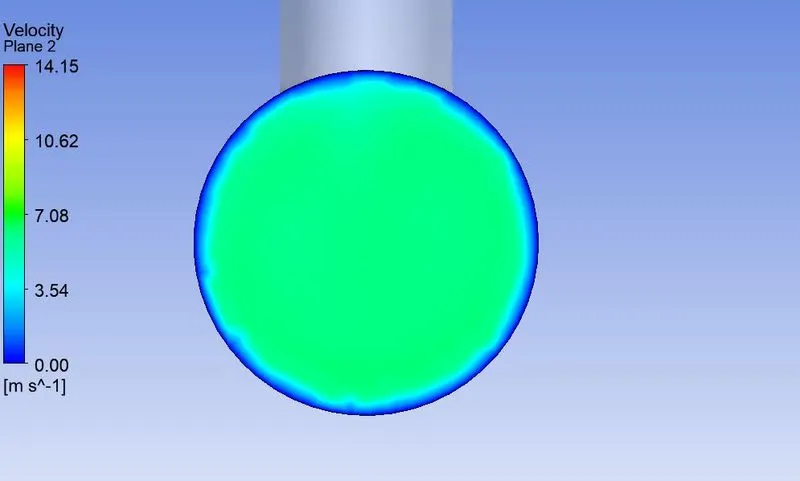
• When hot inlet velocity = 3 m/s and momentum ratio =4

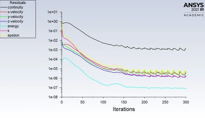
Convergence Plot:

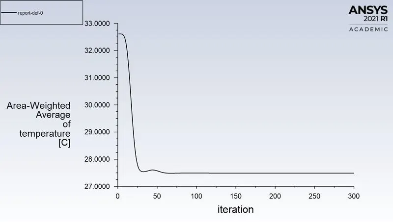
Temperature Plot:

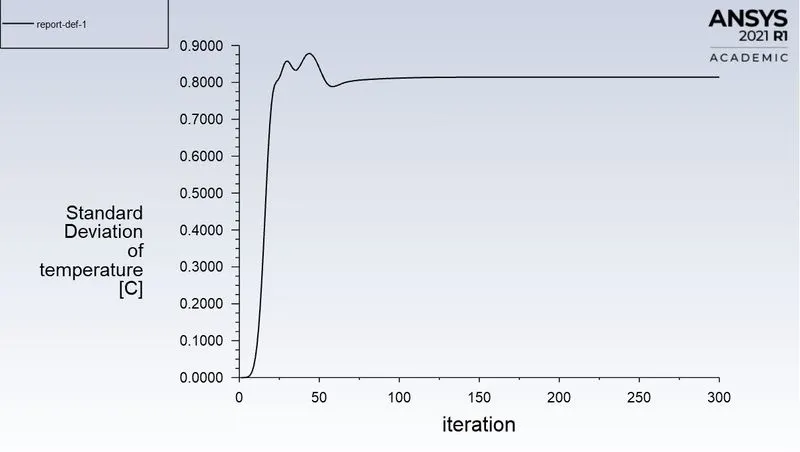
Standard Deviationtion for Temperature:

Velocity Plot:

Contour Plot for Temperature (along the length of fluid flow):

Contour Plot for Temperature (across the length of fluid flow):

Contour Plot for Velocity (along the length of fluid flow):

Contour Plot for Velocity (across the length of fluid flow):

Comparison of 2 cases:

CASE	CELL COUNT	AVERAGE OUTLET TEMPERATURE (ºC)	NUMBER OF ITERATIONS FOR CONVERGENCE
Short Tee with Momentum Ratio 2	105858	30.35	170
Short Tee with Momentum Ratio 4	105858	27.5	160
Long Tee with Momentum Ratio 2	140025	30.4	175
Long Tee with Momentum Ratio 4	140025	27.5	Around 175

Conclusion

1. Mesh Independence Test :We have taken a short mixing tee for this purpose. We performed the simulation for short tee thrice with three different mesh grid sizes. We ran the simulation each time taking mesh sizes 2mm, 3mm and 4mm respectively. Each time the simulation ran, the results are converged at a constant iteration of around 160 and yielded a temperature of approximately 27.5 ºC. It hence shows that the simulation is mesh independent.
2. As we discussed above, since k-epsilon works well with the mixing simulation, it has been chosen for all cases. The k-omega does not seem to predict credible results as it works well, predicting results near the boundaries.
3. Effect of length and momentum ratio on results:In case 1, short tee pipes are simulated with two different momentum ratios 2 and 4. That means, in one of the simulations the velocity of the cold inlet velocity is lesser than the latter one. It is found that, when velocity is more, the mixing effectiveness is improved significantly and desired outlet temperature is obtained. This works the same with case 2, the long tee. Both short tee and long tee, when momentum ratio is more, give similar desired outlet temperature but the number of cells in the case of the long tee is more compared to the short tee which increases the simulation time quadratically. Hence the optimum model is a short tee with a momentum ratio of 4.