Week 7 - Simulation of a 1D Super-sonic nozzle flow simulation using Macormack Method

Simulation Of A 1D Super-Sonic Nozzle Flow Simulation Using Macormack Method

AIM: To simulate the isentropic flow through a quasi 1D subsonic-supersonic nozzle by both the conservation and non-conservation forms of the governing equations and solve them using MacCormack's technique.

OBJECTIVE:

• Perform a grid independence test on the solution and explain all your findings.
• The code must be modular. You need to write separate functions to solve both forms.
• Discuss all the plots you are providing with observed inferences.
• Steady-state distribution of primitive variables inside the nozzle.
• Time-wise variation of the primitive variables.
• Variation of Mass flow rate distribution inside the nozzle at different time steps during the time-marching process.
• Comparison of Normalized mass flow rate distributions of both forms.

THEORY:

In this case steady, isentropic flow through a convergent-divergent nozzle is studied. Inlet of nozzle is connected to the reservoir in which flow is subsonic, at throat flow is sonic and at the outlet flow is supersonic. The ultimate objective of the challenge is to write a MATLAB code that calculated mass flow rate through the nozzle using a conservative and non-conservative form of governing equations. At the later part of the challenge, the error in density, velocity, and temperature at each time step is discussed as well mass flow rate at different time steps for both forms of governing equations.

The total length of the nozzle is taken as 3units in this case first the 1D nozzle is discretized into 31 grid points and gradually increased then grid dependency of mass flow rate is studied for different mesh parameters. By literature review, it's obvious that at a certain point of the time value of velocity, density, the temperature will be constant after a certain point of the time step. So, in this case, initially, tolerance for the above parameters and mass flow rate is taken as 1e-4, and number of time step its taking for convergence for both forms of equations are jotted down then tolerance is varied to 1e-5, 1e-6 and then the number of time steps required for convergence of parameters are studied.

NON-CONSERVATIVE FORM:

Rho - Density

V- Velocity

T - Temperature

t - Time

A - Area

GOVERNING EQUATIONS:

Continuity Equation: `(delrho)/(delt) = - rho*(delV)/(delx) - rho*V*(delln(A))/(delx) - V*(delrho)/(delx)`

Momentum Equation:`(delV)/(delt)=-V*(delV)/(delx) -(1/gamma)*(((delT)/(delx))+(T/rho)*((delrho)/(delx)))`

Energy Equation: `(delT)/(delt)=-V*(delT)/(delx) - (gamma-1)*T[(delV)/(delx)+V(delln(A))/(delx)]`

`BOUNDARY CONDITIONS AT t=0`

`rho = 1-0.3146x`

`T = 1-0.2341x`

`V = (0.1+1.09x)T^(1/2)`

`a = (1 + 2.2(x-1.5)^2)`

INITIAL CONDITIONS:

`V(n) = 2V(n - 1) - V(n - 2)`

`rho(n) = 2rho(n - 1) - rho(n - 2)`

`T(n) = 2T(n - 1) - T(n - 2)`

`V(1) = 2V(2) - V(3)`

`rho(1) = 1`

`T(1) = 1`

TIME STEP CALCULATION:

The most important factor of any simulation is the stability of the solution. It highly depends on the value of time step increments. In this particular case time step can be calculated as:

`deltat=CFL*(deltax)/(a+V)` `

`Where CFL is Courant Friedrichs Lowry (CFL) number which determines the stability highly. Usually value of CFL must be less than 1 or else the solution will blow up as seen in previous challenges. Now, deltax is the distance between each node, a is the velocity of sound and V is local velocity. But velocity value will be changing at point in this challenge so, the minimum value from the above step is used as a time step calculation of the solution. It's noted that for CFL above one solution isn't stable. As well CFL is 0.9 it takes a lot of iteration than usual to converge. Hence 0.5 is idle CFL number for this challenge.`

MACORMACK PROCEDURE:

For instance, assume we are calculating the continuity equation.

• First step in Macromack procedure is to find predictor value which uses forward marching for the taken equation. Which will be:

`(delrho)/(delt)=-rho*(V(i+1)-V(i))/(deltax) - rhoV*(lnA(i+1)-lnA(i))/(deltax) - V*(rho(i+1)-rho(i))/(deltax)`

Similar procedure is done to the momentum and energy eqaution.

• The next step is to update all the three parameters given as boundary conditions for the next time step which can be done as:

`rho(t+deltat) = rho(t) + ((delrho)/(delt)(t)*deltat)`

where density derivative is the one which obtained in previous

• Next step is corrector step which has to be done for the three governing eqauations. In this backward/rearward difference must be used. So corrector step for density dervivative can be calulated as:

`(delrho)/(delt)=-rho*(V(i)-V(i-1))/(deltax) - rhoV*(lnA(i)-lnA(i-1))/(deltax) - V*(rho(i)-rho(i-1))/(deltax)`

and the similar procedure can be followed for velocity and temperature as well.

• Now the derivatives of the parameters obtained from the corrector and predictor value should be averaged and then it should be updated in the next step. Density derivative can be done as:`((delrho)/(delt))avg = 0.5*[((delrho)/(delt))predic + ((delrho)/(delt))cor ]` where predictor and corrector derivative values are obtained from previous two steps

• `The last step is to update the obtained average value of derivative with the value at beginning of the time step by multiplying with deltat and the value is fed as new density for next time step calculation. Final update of density can be done as: ``rho(t+deltat)=rho(t)+((delrho)/(delt))avg*deltat`. This step will be repeated until it reaches a certain convergence`
• The same procedure can be used for conservative form as well just by replacing the governing equations and following the same steps.

The main Advantage of using the MacroMack technique is that it will be using forward difference for predictor step and backward difference for corrector step. Both forward and backward difference methods are first-order approximation which just uses first-order differential equations.

If we go for a second-order central difference scheme it will be having second-order differential equations which take a lot of time for computation. Hence as an order of central difference goes up gradually time for solving too will take so long. So, it doesn’t mean the use of the MacCormack technique (first-order) will yield poor results.

Since it's taking corrector (backward method) and predictor(forward method) for computing and this average value is updated at each time step it will be accurate like the second-order technique but it will take less amount of time than second order because of a lower-order partial differential equation.

CODE AND EXPLANATION:

FUNCTION FOR NON-CONSERVATIVE FORM

• The purpose of the function is to calculate the values of
  Mass flow rate, Pressure, Mach number, Density, velocity, Temperature, Density at the throat, velocity at the throat, Temperature at throat, Mass flow rate at throat, Pressure at throat, Mach number at throat by the known equations for all the grid points.
  
  
• For this initial boundary conditions are established for Density, Temperature & Velocity, and profiles for calculating area & throat.
• Now Outer Time loop is computed for the loop to calculate all the grid points for various formulas inside the loop.
• MacCormack technique is used to solve the numerical solution of governing equations such as Continuity, Momentum & Energy Equation.
• The technique implies two methods for solving namely the Predictor method followed by the Corrector method.
• Predictor & Corrector methods are assigned within the for loop individually for calculating values.
• The calculated values are averaged in the next step and updating the solution with old values.
• Boundary Conditions are applied within the for loop and subsequently used for calculating the Mass Flow Rate, Mach Number & Pressure and also calculating the values throat section.
• Finally plotting is done for Distance(x) & Mass Flow Rate for different Timesteps.
• The program is ended.

function[K,rho,T,v,m_n,Mach_n,p_n,rho_exact_n,T_exact_n,p_exact_n,Mach_exact_n,rho_throat,v_throat,T_throat,p_throat,Mach_throat] = Non_conv(x,n,gamma,nt,dx,dt)
    tic;

    %Inputs
    n = 61;
    x = linspace(0,3,n);
    dx = x(2) - x(1);

    % initial condition
    rho = 1 - 0.3146*x;
    T = 1 - 0.2314*x;
    v = (0.1 + 1.09*x).*T.^2;
    a = 1 + 2.2*(x - 1.5).^2;
    nt = 1400;
    C = 0.5;
    dt = min(C*(dx./(sqrt(T) + v)));
    gamma =1.4;

    throat = find(a==1);
    
    % Outer time loop
    for K = 1:nt
        rho_old = rho;
        v_old = v;
        t_old = T;
     
        for j = 2:n-1
            dv_dx = (v(j+1) -v(j))/dx;
            drho_dx =(rho(j+1) -rho(j))/dx;
            dt_dx = (T(j+1) -T(j))/dx;
            dloga_dx = (log(a(j+1)) -log(a(j)))/dx;

            %continuity eqation
            drho_dt_p(j) = -rho(j)*dv_dx -rho(j)*v(j)*dloga_dx -v(j)*drho_dx;

            %Momentum equation
            dv_dt_p(j) = -v(j)*dv_dx -(1/gamma)*(dt_dx + (T(j)/rho(j))*drho_dx);

            %Energy equation
            dt_dt_p(j) =-v(j)*dt_dx -(gamma-1)*T(j)*(dv_dx + v(j)*dloga_dx);


            rho(j) = rho(j)+drho_dt_p(j)*dt;
            v(j) = v(j) + dv_dt_p(j)*dt;
            T(j) = T(j)+dt_dt_p(j)*dt;
        end

        for j = 2:n-1
            dv_dx = (v(j)-v(j-1))/dx;
            drho_dx =(rho(j)-rho(j-1))/dx;
            dt_dx = (T(j)-T(j-1))/dx;
            dloga_dx = (log(a(j))-log(a(j-1)))/dx;

            %continuity eqation
            drho_dt_c(j) = -rho(j)*dv_dx -rho(j)*v(j)*dloga_dx -v(j)*drho_dx;

            %Momentum equation
            dv_dt_c(j) = -v(j)*dv_dx -(1/gamma)*(dt_dx + (T(j)/rho(j))*drho_dx);

            %Energy equation

            dt_dt_c(j) =-v(j)*dt_dx -(gamma-1)*T(j)*(dv_dx + v(j)*dloga_dx);

        end

        % avg time step
        drho_dt = 0.5*(drho_dt_p+drho_dt_c);
        dv_dt = 0.5*(dv_dt_p+dv_dt_c);
        dt_dt = 0.5*(dt_dt_p+dt_dt_c);

        for i = 2:n-1
        
        rho(i) = rho_old(i) + drho_dt(i)*dt;
        v(i) = v_old(i)+ dv_dt(i)*dt;
        T(i) = t_old(i) + dt_dt(i)*dt;
        end
        
        %inlet BC
        v(1)=2*v(2)-v(3);

        %Outlet BC
        v(n) = 2*v(n-1)-v(n-2);
        rho(n) = 2*rho(n-1)-rho(n-2);
        T(n) = 2*T(n-1)-T(n-2);

        %mass flow rate
        m_n = rho.*a.*v;

        %pressure ratio
        p_n = rho.*T;

        %Mach number
        Mach_n = v./sqrt(T);

        % throat 

        rho_throat(K) = rho(throat);
        v_throat(K) = v(throat);
        T_throat(K) = T(throat);
        p_throat(K) = p_n(throat);
        Mach_throat(K) = Mach_n(throat);


        %Exact solution
        rho_exact_n=0.634*ones(1,1400);
        T_exact_n=0.833*ones(1,1400);
        p_exact_n=0.528*ones(1,1400);
        Mach_exact_n=1*ones(1,1400);

        % plot 
        
        figure(1)
        hold on
        if K==1
            plot(x,m_n,'linewidth',2)
         hold on
        elseif K==50
                plot(x,m_n,'g','linewidth',2)
        hold on
        elseif K==100
                plot(x,m_n,'r','linewidth',2)
        hold on
        elseif K==200
                plot(x,m_n,'c','linewidth',2)
        hold on
        elseif K==700
                plot(x,m_n,'y','linewidth',2)
        hold on
        elseif K==900
                plot(x,m_n,'--','linewidth',2);
            grid on;    
            xlabel('Non-Dimensional Nozzle Dimension');
            ylabel('Non-Dimensional Mass Flow Rate');
            legend('0dt','50dt','100dt','200dt','700dt','900dt')
            title('Mass Flow Rate At Different Time Step')    
        end
   end
   toc;    
 end

FUNCTION FOR CONSERVATIVE FORM

• The purpose of the function is to calculate the values of
  Mass flow rate, Pressure, Mach number, Density, velocity, Temperature, Density at the throat, velocity at the throat, Temperature at throat, Mass flow rate at throat, Pressure at throat, Mach number at the throat by the known equations for all the grid points.
  To determine the initial profile of Density & Temperature, for loop is used inputting the known conditions within an else-if command.
• Initial values of area, throat, velocity & Pressure are calculated using formulas.
• In order to simplify and avoid errors, the equation is split into Solution Vector(U), Flux Vector(F), and Source Term(J).
• Now Outer Time loop is computed for the loop to calculate all the grid points for various formulas inside the loop.
• MacCormack technique is used to solve the numerical solution of governing equations such as Continuity, Momentum & Energy Equation.
• The technique implies two methods for solving namely the Predictor method followed by the Corrector method.
• Predictor & Corrector methods are assigned within the for loop individually for calculating values.
• The calculated values are averaged in the next step and updating the solution with old values.
• Boundary Conditions are applied within the for loop and subsequently used for calculating the Mass Flow Rate, Mach Number & Pressure and also calculating the values throat section.
• Finally plotting is done for Distance(x) & Mass Flow Rate for different Timesteps.
• The program is ended.

function [v_c,rho_c,T_c,m,Mach_c,p,p_c,v_throat,rho_throat,T_throat,m_throat,Mach_throat,p_throat,n,x,nt,dx] = conv(n,x,nt,dx)

tic;
% input variables
n = 61;
x = linspace(0,3,n);
dx = x(2)-x(1);
c = 0.5;
a = 1 + 2.2*(x - 1.5).^2;

%Initial conditions 

for i = 1:n
    if (x(i)>= 0 && x(i)<=0.5)
        rho_c(i) = 1;
        T_c(i) = 1;
    elseif (x(i)>= 0.5 && x(i)<= 1.5)
        rho_c(i) = 1 - 0.366*(x(i) - 0.5);
        T_c(i) = 1 - 0.167*(x(i) - 0.5);
    elseif (x(i)>=1.5 && x(i)<=3.5)
        rho_c(i) = 0.634 - 0.3879*(x(i) - 1.5);
        T_c(i) = 0.833 - 0.3507*(x(i) - 1.5);
    end
end


% steady state flow 
  v_c = 0.59./(rho_c.*a);
  gamma = 1.4;
  throat = find(a==1); 
 
  p = rho_c.*T_c;
  u1 = rho_c.*a;
  u2 = rho_c.*a.*v_c;
  u3 = u1.*((T_c./(gamma-1))+((gamma/2).*(v_c.^2)));

  % timestep
  dt = min (c.*(dx./((T_c.^0.5)+v_c))); 
  nt = 1400;
   
  % Time loop
for k = 1:nt
    
    u1_old = u1;
    u2_old = u2;
    u3_old = u3;

    f1 = u2;
    term1 = (((gamma-1)/gamma)*(u3-((gamma/2)*((u2.^2)./u1))));
    f2 = ((u2.^2)./u1)+ term1;
    f3 = ((gamma*u2.*u3)./u1)-(gamma*(gamma-1)*(u2.^3))./(2*u1.^2);

    % Predictor Method
    for i = 2:n-1
      
        df1_dx(i) = (f1(i+1)-f1(i))/dx;
        df2_dx(i) = (f2(i+1)-f2(i))/dx;
        df3_dx(i) = (f3(i+1)-f3(i))/dx;
        
        da_dx(i) = (a(i+1)-a(i))/dx;
        J2(i) = (1/gamma)*(rho_c(i)*T_c(i))*da_dx(i); 
        
        % continuity equation
        du1_dt_p(i) = -df1_dx(i);
        
        % momentum equation
        du2_dt_p(i) = -df2_dx(i) + J2(i);
        
        % energy equation
        du3_dt_p(i) = -df3_dx(i);
        
        %Solution update
        u1(i) = u1(i) + du1_dt_p(i)*dt;
        u2(i) = u2(i) + du2_dt_p(i)*dt;
        u3(i) = u3(i) + du3_dt_p(i)*dt;    
        
    end
    
    
    % Decoding primitive terms to initialize the corrector step
    rho_c = u1./a;
    v_c = u2./u1;
    T_c = (gamma-1)*((u3./u1)-((gamma*v_c.^2)/2));
    
    % "Pure" form of the flux terms for the corrector step
    f1 = u2;
    term2 = (((gamma-1)/gamma)*(u3-(gamma*u2.^2)./(2*u1)));
    f2 = ((u2.^2)./u1)+ term2;
    f3 = ((gamma*u2.*u3)./u1)-(gamma*(gamma-1)*(u2.^3))./(2*u1.^2);
    
    % Corrector Method
    for i = 2:n-1

        df1_dx(i) = (f1(i)-f1(i-1))/dx;
        df2_dx(i) = (f2(i)-f2(i-1))/dx;
        df3_dx(i) = (f3(i)-f3(i-1))/dx;
        
        da_dx1(i) = (a(i)-a(i-1))/dx;
        J3(i) = (1/gamma)*(rho_c(i)*T_c(i))*da_dx1(i); 
 
        % Continuity equation
        du1_dt_c(i) = -df1_dx(i);
        
        % Momentum equation
        du2_dt_c(i) = -df2_dx(i) + J3(i);
        
        %Energy equation
        du3_dt_c(i) = -df3_dx(i);
        
    end
    
    % Average derivative
    du1_dt = 0.5*(du1_dt_p + du1_dt_c);
    du2_dt = 0.5*(du2_dt_p + du2_dt_c);
    du3_dt = 0.5*(du3_dt_p + du3_dt_c);
    
    % Final solution update
     for j = 2:n-1
        u1(j) = u1_old(j) + du1_dt(j)*dt;
        u2(j) = u2_old(j) + du2_dt(j)*dt;
        u3(j) = u3_old(j) + du3_dt(j)*dt;
     end
     
    % boundary conditions
    % inlet
    u1(1) = rho_c(1)*a(1);
    u2(1) = 2*u2(2) - u2(3);
    v_c(1) = u2(1)/u1(1);
    u3(1) = u1(1)*((T_c(1)/(gamma-1))+((gamma/2)*v_c(1)^2));
    
    % outlet 
    u1(n) = 2*u1(n-1) - u1(n-2);
    u2(n) = 2*u2(n-1) - u2(n-2);
    u3(n) = 2*u3(n-1) - u3(n-2);
    
    rho_c = u1./a; 
    v_c = u2./u1;
    T_c = (gamma-1)*((u3./u1)-((gamma*v_c.^2)/2));
    
    m = rho_c.*v_c.*a;
    Mach_c = v_c./((T_c).^0.5);
    p_c = rho_c.*T_c;
    

    rho_throat(k) = rho_c(throat);
    T_throat(k) = T_c(throat); 
    p_throat(k) = p_c(throat);
    Mach_throat(k) = Mach_c(throat);
    v_throat(k) = v_c(throat);
    m_throat(k) = m(throat);
    
   
    % Plotting 
    figure(2);
    if k  == 50
      plot(x, m, 'b', 'linewidth', 2)
    hold on
     elseif k  == 100
      plot(x, m, 'r', 'linewidth', 2)
    hold on
     elseif k  == 150
      plot(x, m, 'c', 'linewidth', 2)
    hold on
     elseif k  == 200
      plot(x, m, 'g', 'linewidth', 2)
    hold on
     elseif k == 550
      plot(x, m, 'y', 'linewidth', 2) 
    hold on  
     elseif k  == 700
      plot(x, m, 'k', 'linewidth', 2)
    hold on
      elseif k  == 900
      plot(x, m,'m', 'linewidth', 2)
      
     grid on
     ylabel('Non-Dimensional Mass Flow Rate');
     xlabel('Non-Dimensional Distance Through Nozzle(x)');
     title('Variation Of Mass Through Nozzle At Different Time teps')
     legend({'50 time steps','100 time steps','150 time steps','200 time steps','550 time steps','700 time steps','900 time steps'});
   end     
end
toc;
end

MAIN CODE:

• We start the program by considering the required inputs n, x, dx, gamma, nt.
• Non-Conservative and Conservative forms are created as separate functions with the necessary inputs
• tic toc command is used for calculating the time elapsed between the functions.
• Plotting: 1. Steady-state distribution of primitive variables inside the nozzle.
  2. Time-wise variation of the primitive variables.
  3. Variation of Mass flow rate distribution inside the nozzle at different time steps during the time-marching process.
  4. Comparison of Normalized mass flow rate distributions of both forms.
• Each plot is computed as subplots of four primitive variables such as Density, Temperature, Pressure, and Mach Number at the throat as well as Convergent/Divergent section.

clear all
close all
clc
% Inputs
n = 61;
x = linspace(0,3,n);
dx = x(2) - x(1);
gamma = 1.4;
nt = 1400;

tic;
[K,rho,T,v,m_n,Mach_n,p_n,rho_exact_n,T_exact_n,p_exact_n,Mach_exact_n,rho_throat,v_throat,T_throat,p_throat,Mach_throat] = Non_conv(x,n,gamma,nt,dx);
Non_conservative_time = toc;

tic;
[v_c,rho_c,T_c,m,Mach_c,p,p_c,v_throat,rho_throat,T_throat,m_throat,Mach_throat,p_throat,n,x,nt,dx] = conv(n,x,nt,dx);
Conservative_time = toc;

% Conservative form Time wise variation of density,pressure,temperature & Mach numer
figure(6)
subplot(4,1,1)
plot(rho_throat)
hold on
plot(rho_exact_n)
xlabel('Time step')
ylabel('rho/{rho_0}')
title('Time wise variation of density,temperature,pressure and Mach No. at the nozzle throat')
legend('Time wise variation','Exact solution')

subplot(4,1,2)
plot(T_throat)
hold on
plot(T_exact_n)
xlabel('Time step')
ylabel('T/{T_0}')
legend('Time wise variation','Exact solution')

subplot(4,1,3)
plot(p_throat)
hold on
plot(p_exact_n)
xlabel('Time step')
ylabel('p/{p_0}')
legend('Time wise variation','Exact solution')

subplot(4,1,4)
plot(Mach_throat)
hold on
plot(Mach_exact_n)
xlabel('Time step')
ylabel('Mach no')
legend('Time wise variation','Exact solution')
% Non-Conservative form Time wise variation of density,pressure,temperature & Mach numer
figure(5)
subplot(4,1,1)
plot(rho_throat)
hold on 
plot(rho_exact_n)
xlabel('Time step')
ylabel('rho/{rho_0}')
legend('Time wise variation','Exact solution')
title('Time wise variation of density,temperature,pressure and Mach No. at the nozzle throat')


subplot(4,1,2)
plot(T_throat)
hold on 
plot(T_exact_n)
xlabel('Time step')
ylabel('T/{T_0}')
legend('Time wise variation','Exact solution')

subplot(4,1,3)
plot(p_throat)
hold on 
plot(p_exact_n)
xlabel('Time step')
ylabel('p/{p_0}')
legend('Time wise variation','Exact solution')

subplot(4,1,4)
plot(T_throat)
hold on 
plot(T_exact_n)
xlabel('Time step')
ylabel('Mach no')
legend('Time wise variation','Exact solution')


% Non-Conservative vs Conservative form mass flow rate
figure(4)
plot(x,m_n,'r','linewidth',2)
hold on
plot(x,m,'k','linewidth',2)
xlabel('x/L')
ylabel('Non-dimensional mass flow rate')
legend('non-conservative flow','Conservative flow')
grid on;

% Qualitative aspects of 1D nozzle flow
figure(3)
subplot(4,1,3)
plot(x,rho,'r')
hold on
plot(x,rho_c,'*')
xlabel('Length of the nozzle')
ylabel('Density')
legend('Non-conservative','conservative')
grid on;

subplot(4,1,4)
plot(x,T,'r')
hold on
plot(x,T_c,'*')
xlabel('Length of the nozzle')
ylabel('Temperature')
legend('Non-conservative','conservative')
grid on;

subplot(4,1,1)
plot(x,Mach_n,'r')
hold on
plot(x,Mach_c,'*')
xlabel('Length of the nozzle')
ylabel('Mach number')
legend('Non-conservative','conservative')
title('Qualitative aspects of quasi-1D nozzle flow')
grid on;

subplot(4,1,2)
plot(x,p_n,'r')
hold on
plot(x,p_c,'*')
xlabel('Length of the nozzle')
ylabel('Mach number')
legend('Non-conservative','conservative')
grid on;

GRAPHS AND RESULTS:

VARIATION FLOW THROUGHOUT THE NOZZLE:

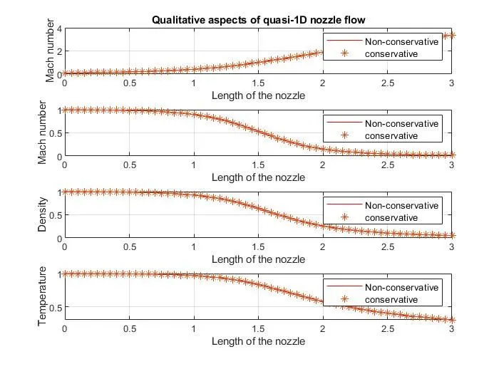
We see in the bellow graph that both conservative and non-conservative are approximately similar at which the steady-state is almost obtained and the values of the primitive variables are in good approximation with the exact analytical solution.

TIMEWISE VARIATION OF FLOW PARAMETER ALONG THE NON-DIMENSIONAL LENGTH OF NOZZLE AT THROAT

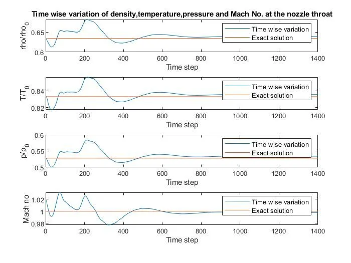
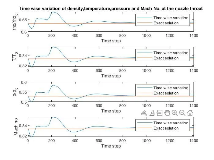
It can be found that the solution of the non-conservative form lies closer to the exact values of rho', 'T', 'p', and 'Mach' when compared to the conservative form solution. Tracking the values of flow parameters at a particular region is a good way of investigating the attainment of the steady-state by the system. The non-conservative form generates more accurate results for the primitive variables. But even after 900 to 1000 time steps difference between the numerical solution and the exact solution exists. For a non-conservative form, the value of difference between the numerical solution and the exact solution will be almost constant after 900 to 1000 time steps and equal to 10^-6. For a conservative form, the value of difference between the numerical solution and the exact solution will be almost constant after 900 to 1000 time steps and equal to 10^-3. From the plots below, it can be seen that the steady-state is almost obtained with a good level of approximation, after 500-time steps for practical purposes. But this evidence is not enough to justify our observation. For further investigation, we are going to observe the mass flow rate (non-dimensional) behavior along the non-dimensional distance 'x' at different steps.

CONSERVATIVE FORM

NON-CONSERVATIVE FORM

NON-DIMENSIONAL MASS FLOW RATE BEHAVIOUR ALONG NON-DIMENSIONAL LENGTH OF NOZZLE

NON-CONSERVATIVE FORM

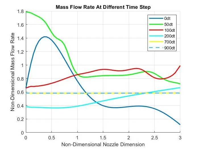
Analyzing the below fig, it can be observed that the mass flow rate curve obtained above 700 and 900-time steps is almost overlying in the same region of space. So this plot substantiates our previous assumption from the observation of the "Timewise variation of flow parameters at the nozzle throat", i.e after 500 time steps almost steady state is obtained (for practical purposes) for the non-conservative form of the flow equations. Theoretically, it takes infinite time steps to attain a steady-state.

CONSERVATIVE FORM

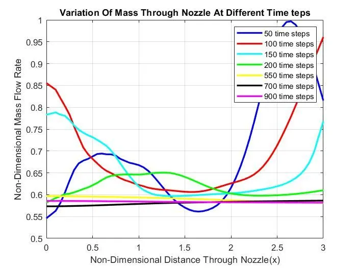
When compared to the previous plot, the fluctuations are less severe in the conservative form. But comparing these two plots makes no sense because we assumed different sets of initial conditions. Therefore we made a guess while choosing the initial conditions(density, temperature, velocity) with constant mass flow, for the conservative form because of its sense of the stability behavior. This is the reason for its mild fluctuating behavior. From the plot, it can be observed that the mass flow rate curve obtained for 550 and 700 and 900-time steps are almost overlying in the same region of space. But, the reasonable settlement of the fluctuations at the 550th time step may be due to the more realistic initial conditions with constant mass flow, assumed by the intelligent guess. And also for the conservative form, the value of residue at the 550th-time step will be somewhere between 10^-1(Initially) and 10^-3(after 900 timesteps), which doesn't lead to a good approximation with the exact solution. i.e in other words, at the 550th-time step, milder fluctuations still exist, which can't be approximated with the exact solution at a good level of accuracy, due to the presence of large values of residue. After 700-time steps, it almost (but not quite) becomes equal to a constant value. Moreover, it is quite close to the exact analytical solution of 0.579, and therefore the steady-state is almost obtained. Theoretically, it takes infinite time steps to attain a steady-state.

COMPARISION OF MASS FLOW RATE OF NON-CONSERVATIVE FORM AND CONSERVATIVE FORM

The conservative form generates a better mass flow distribution with fewer fluctuations when compared with the non-conservative form. The reason is the mass flow itself is one of the dependent variables in the equations of the conservative form, whereas in the non-conservative form, the dependent variables are the primitive variables and the mass flow is obtained after some calculation.

The conservative form generates more accurate results for the flux variables.

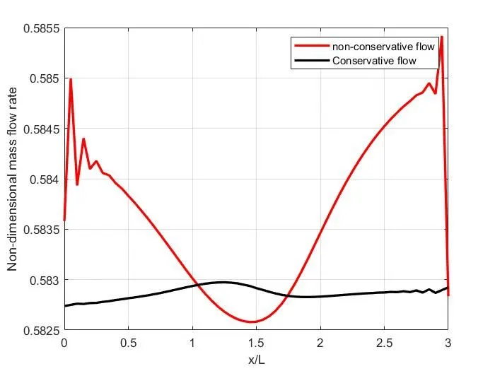
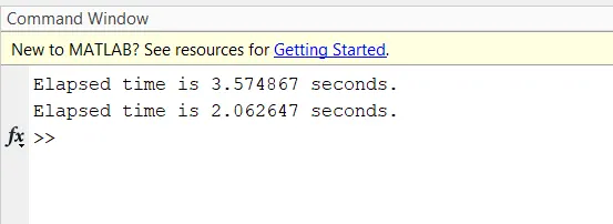
By concluding, In the case of a conservative form, primitive variables need to be decoded from the flux variables, but this is not necessary in the case of a non-conservative form. And therefore solving conservative form requires more computational effort.

SNAP OF COMMAND WINDOW

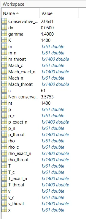
SNAP OF WORKSPACE