Week 3.5 - Deriving 4th order approximation of a 2nd order derivative using Taylor Table method

Deriving 4th Order Approximation Of A 2nd Order Derivative Using Taylor Table Method

AIM: Write a program in Matlab to evaluate the second-order derivative of the analytical function exp(x)*cos(x) and compare it with the 3 numerical approximations that you have derived.

OBJECTIVE:

Derive the following 4th order approximations of the second-order derivative.

1. Central difference

2. Skewed right-sided difference

3. Skewed left-sided difference

and

After deriving these schemes, prove that your skewed schemes are fourth-order accurate i.e the thumb rule given in Once you have done this, write a program in Matlab to evaluate the second-order derivative of the analytical function exp(x)*cos(x) and compare it with the 3 numerical approximations that you have derived. Provide a plot that compares the absolute error between the above-mentioned schemes In your own words, describes why a skewed scheme is useful? What can a skewed scheme do that a CD scheme cannot?

The Report is divided into types one theoretical by numerical derivation and one more is by coding.

First part: Theoretical

1. Central Difference Method:

n = A + O - 1`

where,

n = Number of nodes in stencil

A = Accuracy of the approximation method

O = Order of the numerical function

Here, in our case A = 4; O = 2

So , n = 4+2 -1= 5

Therefore we need 5 nodes in order to find the 2nd order derivative with the 4th order of approximation.

Consider the value of `(del^2y)/(delx^2)` with the 4th order of approximation is given by the equation

`(del^2y)/(delx^2) = af(i - 2) + bf(i - 1) + cf(i) + df(i + 1) + ef(i + 2)`

`dx^2 f''(i)`	f(i)	f'(i)dx	`f''(i)dx^2`	`f'''(i)dx^3`	`f''''(i)dx^4`
af(i-2)	a	-2a	2a	`-(4a)/3`	`(2a)/3`
bf(i-1)	b	-b	`b/2`	`-b/6`	`b/24`
cf(i)	c	0	0	0	0
df(i+1)	d	d	`d/2`	`d/6`	`d/24`
ef(i+2)	e	2e	2e	`(4e)/3`	`(2e)/3`
sum of co_efficients	0	0	1	0	0

This table transform into matrix of type AX=B

`[[1,1, 1, 1, 1],[-2, -1, 0, 1, 2],[ 4/2, 1/2, 0, 1/2, 4/2],[1,2,3,4,5],[-8/6, -1/6,0,1/6,8/6],[16/24 ,1/24,0,1/24,16/24]]` * `[[a],[b],[c],[d],[e]]` = `[[0],[0],[1],[0],[0]]`

on further solving we get the values of the unknown

i.e. Values = a = -0.0833 b= 1.3333 c= -2.5000 d= 1.3333 e= -0.0833

substituting these coefficient in equation we get,

`(del^2u)/(delx^2) = ((-0.0833)f(i-2)+(1.3333)f(i-1)+(-2.5000)f(i)+(1.3333)f(i+1)+(-0.0833)f(i+2))/dx^2`

2.SKEWED RIGHT-HAND DIFFERENCE SCHEME:

So for a skewed scheme, the number of node points are,

n = A+O

n = 4+2

n = 6

We need 6 number of points are required to calculate the fourth-order skewed right side approximation.

Therefore, Consider the value of `(del^2y)/(delx^2)` with the 4th order of approximation is given by the equation

`(del^2y)/(delx^2) = af(i) + bf(i + 1) + cf(i +2 ) + df(i + 3) + ef(i + 4) + gf(i + 5)`

`dx^2 f''(i)`	f(i)	f'(i)dx	`f''(i)dx^2`	`f'''(i)dx^3`	`f''''(i)dx^4`	`f'''''(i)dx^5`
af(i)	a	0	0	0	0	0
bf(i+1)	b	b	`b/2`	`b/6`	`b/24`	`b/120`
cf(i+2)	c	2c	`(4c)/2`	`(8c)/6`	`(16c)/24`	`(32c)/120`
df(i+3)	d	3d	`(9d)/2`	`(27d)/6`	`(81d)/24`	`(243d)/120`
ef(i+4)	e	4e	`(16e)/2`	`(64e)/6`	`(256e)/24`	`(1024e)/120`
gf(i+5)	g	5g	`(25g)/2`	`(125g)/6`	`(625g)/24`	`(3125g)/120`
sum of co_efficients	0	0	1	0	0	0

table are solved using matrix inversion method,

A.X = B

`[[1,1,1,1,1,1],[0,1,2,3,4,5],[0,1/2,4/2,9/2,16/2,25/2],[0,1/6,8/6,27/6,64/6,125/6],[0,1/24,16/24,81/24,256/24,625/24],[0,1/120,32/120,243/120,1024/120,3125/120]].[[a],[b],[c],[d],[e],[g]] = [[0],[0],[1],[0],[0],[0]]`

on further solving we get the values of the unknown i.e.

Values = a = 3.7500 b = -12.8333 c = 17.8333 d = -13.0000 e = 5.0833 f = -0.8333

substituting these coefficient in equation we get,

`(del^2u)/(delx^2) = ((3.7500)f(i)+(-12.8333)f(i+1)+(17.8333)f(i+2)+(-13.0000)f(i+3)+(5.0833)f(i+4)+(-0.8333)f(i+5))/dx^2`

3. SKEWED LEFT HAND DIFFERENCE SCHEME:

For a skewed scheme, the number of node points is

n = A+O

n = 4+2

n = 6

We have 6 number of points are required to calculate the fourth-order left side skewed approximation.

Therefore, Consider the value of `(del^2y)/(delx^2)` with the 4th order of approximation is given by the equation

`(del^2y)/(delx^2)=af(i)+bf(i-1)+cf(i-2)+df(i-3)+ef(i-4)+gf(i-5)`

`dx^2 f''(i)`	f(i)	f'(i)dx	`f''(i)dx^2`	`f'''(i)dx^3`	`f''''(i)dx^4`	`f'''''(i)dx^5`
af(i-5)	a	-5a	`(25a)/2`	`-(125a)/6`	`(625a)/24`	`-(3125a)/120`
bf(i-4)	b	-4b	`(16b)/2`	`-(64b)/6`	`(256b)/24`	`-(1024b)/120`
cf(i-3)	c	-3c	`(9c)/2`	`-(27c)/6`	`(81c)/24`	`-(243c)/120`
df(i-2)	d	-2d	`(4d)/2`	`-(8d)/6`	`(16d)/24`	`-(32d)/120`
ef(i-1)	e	-e	`e/2`	`-e/6`	`e/24`	`-e/120`
gf(i)	g	0	0	0	0	0
sum of co_efficients	0	0	1	0	0	0

table are solved using matrix inversion method

A.X = B

`[[1,1,1,1,1,1],[-5,-4,-3,-2,-1,0],[25/2,16/2,9/2,4/2,1/2,0],[-125/6,-64/6,-27/6,-8/6,-1/6,0],[625/24,256/24,81/24,16/24,1/24,0],[-3125/120,-1024/120,-243/120,-32/120,-1/120,0]].[[a],[b],[c],[d],[e],[g]] = [[0],[0],[1],[0],[0],[0]]`

on further solving we get the values of the unknown i.e.

Values = a = -0.8333 b = 5.0833 c =13.0000 d = 17.8333 e = -12.8333 f = 3.7500

substituting these coefficient in equation we get

`(del^2u)/(delx^2) = ((-0.8333)f(i-5)+(5.0833)f(i-4)+(-13.0000)f(i-3)+(17.8333)f(i-2)+(-12.8333)f(i-1)+(3.7500)f(i))/dx^2`

METHOD BY CODING:

Main code:

Explanation

• We start by creating the function file separately for different approximation techniques.
• In the function file, assign the input variables of the respective approximation schemes. Additionally, write the respective matrix for the particular scheme in order to find coefficients of the resulting approximation equations.
• Insert formula of the respective approximation scheme individually in different schemes and as an output to calculate the fourth-order error incurred in that dedicated approximation scheme.
• Then define the input parameters like the value of "x", "range of dx" using linspace command, and "second-order derivative of the analytical function.
• Create a for loop to calculate the error along with dx, 200 being the number of intervals across the range of "dx'. Errors pertaining to the central, skewed right side, and skewed left side approximation schemes will be calculated inside the loop resulting in an array of 200 steps along with the "dx".
• After calculating the errors, plot them using "loglog" command as it gives results in the logarithmic 10 base scale, which will facilitate interpreting results.
• Finally, insert the title, legend, and labels to display results in an effective manner.

clear all
close all
clc

%Input values for the program
x= pi/3;

dx= linspace(pi/4,pi/4000,20);

for i=1:length(dx)
    
    central_differencing(i) = CD_fourth_order(x,dx(i));
    
    Skewed_right_sided(i) = RS_fourth_order(x,dx(i));
    
    Skewed_left_sided(i) = LS_fourth_order(x,dx(i));
    
end

% Plotting

figure(1)
loglog(dx,central_differencing,'g')
hold on
loglog(dx,Skewed_right_sided,'r')
hold on
loglog(dx,Skewed_left_sided,'b')
xlabel('range of dx')
ylabel('Error')
title('range of dx vs error')
legend('central differencing','skewed right sided difference','skewed left sided difference')

Code for Central Differencing Method:

function Central_diff_error = CD_fourth_order(x,dx)

% analytic function 
analytical_derivative = -2*exp(x)*sin(x);

%central differencing
central_diff = (((-0.0833)*((exp(x-(2*dx)))*(cos(x-(2*dx)))))+((1.3333)*((exp(x-dx))*(cos(x-dx))))-((2.5000)*((exp(x))*(cos(x))))+((1.3333)*((exp(x+dx))*(cos(x+dx))))-((0.0833)*((exp(x+(2*dx)))*(cos(x+(2*dx))))))/(dx^2);

%error
Central_diff_error = abs(central_diff- analytical_derivative);
end

Code for Skewed Right-sided differencing Method:

function Right_sided_skewed_error = RS_fourth_order(x,dx)

% analytic function 
analytical_derivative = -2*exp(x)*sin(x);

% Skewed Right-sided
right_sided_skewed = (((3.7500)*((exp(x))*(cos(x))))-((12.8333)*((exp(x+dx))*(cos(x+dx))))+((17.8333)*((exp(x+(2*dx)))*(cos(x+(2*dx)))))-((13.0000)*((exp(x+(3*dx)))*(cos(x+(3*dx)))))+((5.0833)*((exp(x+(4*dx)))*(cos(x+(4*dx)))))-((0.8333)*((exp(x+(5*dx)))*(cos(x+(5*dx))))))/(dx^2);

%error
Right_sided_skewed_error = abs(right_sided_skewed - analytical_derivative);
end

Code for Skewed Left-sided differencing Method:

function Left_sided_skewed_error = LS_fourth_order(x,dx)

% analytic function 
analytical_derivative = -2*exp(x)*sin(x);

% Skewed Left side
left_sided_skewed = (((-0.8333)*((exp(x-(5*dx)))*(cos(x-(5*dx)))))+((5.0833)*((exp(x-(4*dx)))*(cos(x-(4*dx)))))-((13.0000)*((exp(x-(3*dx)))*(cos(x-(3*dx)))))+((17.8333)*((exp(x-(2*dx)))*(cos(x-(2*dx)))))-((12.8333)*((exp(x-dx))*(cos(x-dx))))+((3.7500)*((exp(x))*(cos(x)))))/(dx^2);

%error
Left_sided_skewed_error = abs(left_sided_skewed - analytical_derivative);
end

RESULTS:

We conclude the above comparison of absolute error for the left, right and central differencing scheme can be seen in the below graph. The graph shows that the central scheme is most accurate compared to the skewed differencing. The curves also show that when the value of dx is very small or large the approximating function becomes unstable.

Sometimes for a wider range of step size, higher-order approximation techniques stood out to be inefficient as the error at any point is the net sum of a numerical error and round-off error. Higher-order approximation techniques have a high value of round-off error, so in such instances lower order approximation techniques are preferred for the accuracy of the solution.

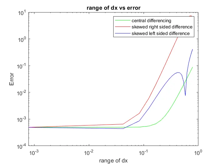
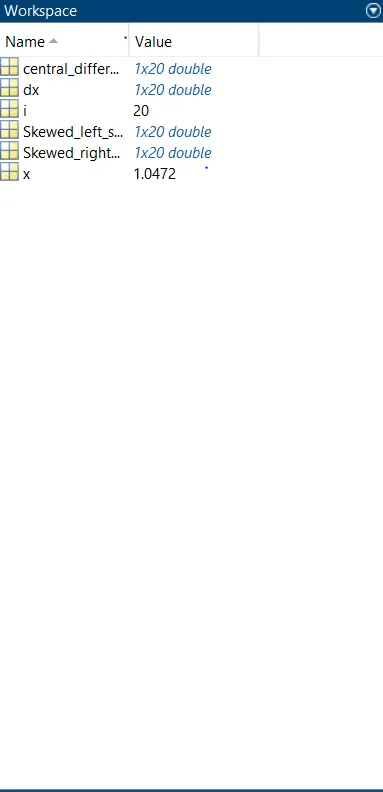
Image of the workspace

• Why skewed scheme is useful? What can a skewed scheme do that a central differencing scheme cannot?

The central difference approximation scheme takes information from both the sides of the node point which to be evaluated i.e. in an asymmetric manner. However, skewed schemes extract information from either side of the nodal position (It can be left or right). When the function or a nodal point is to be evaluated in space or domain, where it might have nodal points only in one direction i.e. either in right or left. In such instances, skewed schemes are preferred over central approximation schemes. Though the central difference approximation scheme is more significant in terms of accuracy still it loses its stance when it comes to calculating a function at the boundary of a domain.

Central Differencing Method can not be employed at the boundary nodes due to the unavailability of right and left nodes at the same time. In such cases, the skewed differencing scheme is used.