Simulation of a 1D Super-sonic Nozzle flow by MacCormack Method using MATLAB
Week 7 Report.
- Aim: To simulate the isentropic flow through a quasi 1D subsonic-supersonic nozzle using the Conservation and the Non-Conservation form of the Governing Equations and solving them by using the Macormack method.
- Theoretical Intoruction:
Isentropic nozzle flow describes the movement of a gas or fluid through a narrowing opening without an increase or decrease in entropy.
Whenever a gas is forced through a tube, the gaseous molecules are deflected by the tube's walls. If the speed of the gas is much less than the speed of sound, the gas density will remain constant and the velocity of the flow will increase. However, as the speed of the flow approaches the speed of sound, compressibility effects on the gas are to be considered. The density of the gas becomes position dependent. While considering flow through a tube, if the flow is very gradually compressed (i.e. area decreases) and then gradually expanded (i.e. area increases), the flow conditions are restored (i.e. return to its initial position). So, such a process is a reversible process. According to the Second Law of Thermodynamics, whenever there is a reversible and adiabatic flow, constant value of entropy is maintained. Engineers classify this type of flow as an isentropic flow of fluids. Isentropic is the combination of the Greek word "iso" (which means - same) and entropy.
When the change in flow variables is small and gradual, isentropic flows occur. The generation of sound waves is an isentropic process. A supersonic flow that is turned while there is an increase in flow area is also isentropic. Since there is an increase in area, therefore we call this an isentropic expansion. If a supersonic flow is turned abruptly and the flow area decreases, the flow is irreversible due to the generation of shock waves. The isentropic relations are no longer valid and the flow is governed by the oblique or normal shock relations.
A de Laval nozzle (or convergent-divergent nozzle, CD nozzle or con-di nozzle) is a tube that is pinched in the middle, making a carefully balanced, asymmetric hourglass shape. It is used to accelerate a hot, pressurized gas passing through it to a higher supersonic speed in the axial (thrust) direction, by converting the heat energy of the flow into kinetic energy. Because of this, the nozzle is widely used in some types of steam turbines and rocket engine nozzles. It also sees use in supersonic jet engines.
A de Laval nozzle will only choke at the throat if the pressure and mass flow through the nozzle is sufficient to reach sonic speeds, otherwise no supersonic flow is achieved, and it will act as a Venturi tube; this requires the entry pressure to the nozzle to be significantly above ambient at all times (equivalently, the stagnation pressure of the jet must be above ambient).
In addition, the pressure of the gas at the exit of the expansion portion of the exhaust of a nozzle must not be too low. Because pressure cannot travel upstream through the supersonic flow, the exit pressure can be significantly below the ambient pressure into which it exhausts, but if it is too far below ambient, then the flow will cease to be supersonic, or the flow will separate within the expansion portion of the nozzle, forming an unstable jet that may "flop" around within the nozzle, producing a lateral thrust and possibly damaging it.
In practice, ambient pressure must be no higher than roughly 2–3 times the pressure in the supersonic gas at the exit for supersonic flow to leave the nozzle.
In accordance with conservation of mass the mass flow rate of the gas throughout the nozzle is the same regardless of the cross-sectional area.

where: 
= mass flow rate, 
= cross-sectional area of the throat, 
= total pressure, 
= total temperature, 
 = isentropic expansion factor,
= gas constant, 
= Mach number 
= the gas molecular mass
When the throat is at sonic speed Ma = 1 where the equation simplifies to:

By Newtons third law of motion the mass flow rate can be used to determine the force exerted by the expelled gas by:

where: 
= force exerted, = mass flow rate, 
= exit velocity at nozzle exit In aerodynamics, the force exerted by the nozzle is defined as the thrust.
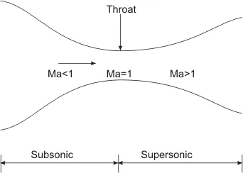
Convergent-Divergent Nozzle
MacCormack Method: In computational fluid dynamics, the MacCormack method is a widely used discretization scheme for the numerical solution of hyperbolic partial differential equations. This second-order finite difference method was introduced by Robert W. MacCormack in 1969. The MacCormack method is elegant and easy to understand and program. The MacCormack method is well suited for nonlinear equations. The order of differencing can be reversed for the time step (i.e., forward/backward followed by backward/forward). For nonlinear equations, this procedure provides the best results. For linear equations, the MacCormack scheme is equivalent to the Lax–Wendroff method.The MacCormack method is a variation of the two-step Lax–Wendroff scheme but is much simpler in application. To illustrate the algorithm, consider the following first order hyperbolic equation
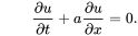
The application of MacCormack method to the above equation proceeds in two steps; a predictor step which is followed by a corrector step.
Predictor step: In the predictor step, a "provisional" value of u at time level `u_i^(n+1)`is estimated as follows

The above equation is obtained by replacing the spatial and temporal derivatives in the previous first order hyperbolic equation using forward differences.
Corrector step: In the corrector step, the predicted value `u_i^(n+1)` is corrected according to the equation

Note that the corrector step uses backward finite difference approximations for spatial derivative. The time-step used in the corrector step is `(Delta t)/2` in contrast to the `delt` used in the predictor step.
Replacing the `u_i^(n+1/2)` term by the temporal average
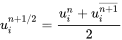
to obtain the corrector step as

- Code/Logic:
1. We firstly need to clear and close all the previously entered codes and the present values of the already used variables, hence we use the following commands:
clear all
close all
clc
2. We start the Main code by giving the necessary inputs such as the number of nodes in which we need to length of the Nozzle to be divided. We also use the linspace command to divide the entire length of the nozzle (3m in our case) into the number of nodes that we have decided to divide. Here we can also specify the distance between two points by simply subtracting the third value of the 'x' array with the second value of the same array. This value of dx will remain constant throughout the entire length of the nozzle. Here is the syntax for the linspace command and all the inputs that we need to make the further calculations.
Syntax for the linspace command:
%Syntax for the Linspace command y = linspace(x1,x2) y = linspace(x1,x2,n)
All the Inputs that we have used:
%Inputs: n=31; %Number of points in the Nozzle x=linspace(0,3,n); %Dividing the Nozzle according to the Number of points dx = x(2)-x(1); %Distance between consecutive points. gamma = 1.4; %Specific Heat Ratio for Standard Air. C = 0.5; %Courant Number.
3. After giving the inputs, we then go on to create seperate functions for the Non-conservation and the Conservation form of the Governing Equations for this simulation.
Firstly, we create a function for the Non-conservation form, the initial condition calculations are done as shown:
rho= 1 - 0.3146*x; %Non-Dimensionalised Density Value T = 1 - 0.2314.*x; %Non-dimensionalised Temperature Value. v = (0.1 + 1.09*x).*(T.^0.5); %Non-dimensionalised Velocity Value.
These are the Initial conditions for this simulation. After this, we then go on to plot the Area profile and then finally go to calculate the Time-Step for the calculations as shown.
To calculate the Time- Step, we firstly need to calculate the Speed of Sound with respect to Temperature that we have calculated in the Initial Conditions. Then, we use this Speed of sound to extract the minimum of all the time-steps that we measure. This minimum value of the time-step is the Time-Step that we need to use for the simulation of the Convergent-Divergent Nozzle.
Like this, we can define the Time-Step for the Convergent-Divergent Nozzle.%Calculating the Speeed of Sound. a = T.^0.5; %Speed of Sound wrt to the Temperature. %Defining the Time-steps according to Speed of sound and velocity of flow. for i=1:length(a) dt1(i) = C*(dx/(a(i)+v(i))); end %Final Time-Step is taken as the minimum value of the dt1 variable that we created. dt = min(dt1);
4.We then go on to create the Outer Time-Loop and now we need to calculate the `((delrho)/dt)_p` ,`((delT)/dt)_p, ((delv)/dt)_p`
These values are just calculated for the Predictor Step as we do in the Macormack method.
Then the Solution update must occur for the Predictor step, this is done by updating the initial conditions using the formula given below:
%Solution Update within the Time-Loop v(j) = v(j) + dvdt_p(j)*dt; rho(j) = rho(j) + drhodt_p(j)*dt; T(j) = T(j) + dTdt_p(j)*dt; The key point to note is that in the Predictor Step, we have the Forward Difference method when calculating the gradients of the primitive variables.
But as we proceed to compute the Corrector steps for the same, we then use the Rearward Difference approach and then again compute the average of the two.
5. Next we compute the variables in the Corrector step. To do this, we must again compute the variables using the Rearward Difference and then compute the average of the variables that we calculated in the Predictor and the Corrector step.
The corrector step is shown below:for j = 2:(n-1) drhodx(j) = (rho(j)-rho(j-1))/(dx); dvdx(j) = (v(j)- v(j-1))/(dx); dTdx(j) = (T(j)-T(j-1))/(dx); dlogadx(j) = (log(A(j))-log(A(j-1)))/(dx); %Calling the Navier-Stokes Equation Function to calculate [drhodt_c(j),dvdt_c(j),dTdt_c(j)]=NSE(rho(j),dvdx(j),v(j),dlogadx(j),drhodx(j),dTdx(j),gamma,T(j)); end
The NSE function is shown below:function [a,b,c] = NSE(rho,dvdx,v,dlogadx,drhodx,dTdx,gamma,T) %Continuity Equation: drhodt = -rho*dvdx - rho*v* dlogadx - v*drhodx; %Momentum Equation: dvdt = -v* dvdx - (1/gamma)*(dTdx+ (T/rho)*drhodx); %Energy Equation: dTdt = -v*dTdx -(gamma-1)*T*(dvdx+ v*dlogadx); a= drhodt; b=dvdt; c=dTdt; end
Now that we have both the Predictor and the Corrector step values calculated, we can proceed to calculate the Average of these two and then doing the final solution update.%Example of the Average Value calculation drhodt = 0.5*(drhodt_p + drhodt_c);
Similarly we can calculate the Average value for all the other two values as well and then proceed to do the Final Solution update. The final solution update is also shown below:%Final Update of the Variables: for i=2:n-1 v(i)= v_old(i) + dvdt(i)*dt; rho(i)= rho_old(i) + drhodt(i)*dt; T(i) = T_old(i) + dTdt(i)*dt; end
6. The final Step is to provide the Boundary conditions at the Inlet and the Outlet of the Nozzle. These Boundary conditions are very important and can affect the entire Simulation.%Applying Boundary Conditions at the Inlet: v(1) = 2*v(2) - v(3); %Applying the Boundary Conditions at the Outlet: v(n) = 2*v(n-1) - v(n-2); rho(n) = 2*rho(n-1) - rho(n-2); T(n) = 2*T(n-1) - T(n-2); m_ncs = rho.*A.*v; %Calculating the Mass Flow Rates. M = v./(T).^0.5; %Calculating the Mach Number.
7. After the Boundary Conditions were given, we then proceed to plot the necessary graphs that we need to study from the 1D Subsonic-Supersonic Nozzle Flow problem that we just solved.
All these graphs can be plotted using the plot command, whose syntax is shown below:plot(X,Y) plot(X,Y,LineSpec) plot(X1,Y1,...,Xn,Yn) plot(X1,Y1,LineSpec1,...,Xn,Yn,LineSpecn) plot(Y) plot(Y,LineSpec) plot(___,Name,Value) plot(ax,___) h = plot(___)All these Syntaxes can be used according to our need and our inputs.
Since, we want to understand how the Primitive Variables are changing with time, we have a seperate plot for it. Another Plot is where we wish to see how these variables change with respect to the different time-steps.
We also, wish to study the how the Mass-Flow rate for a particular form of the Governing Equation is varying at certain time-steps, hence, a seperate plot for it, where the logic that I have used is such that when the value of the Time loop counter hits a particular value, the plots are made for the Distance along the nozzle versus the mass-flow rate calculated at that time-step. The code is shown in the Function shown below.
a. Main-Codeclear all close all clc %Inputs: n=31; %Number of grid points on the Nozzle x=linspace(0,3,n); %Dividing the Nozzle according to the Number of points dx = x(2)-x(1); %Distance between consecutive points. gamma = 1.4; %Specific Heat Ratio for Standard Air. C = 0.5; %Courant Number. %Writing a function for the Non-Conservation Form of the Navier-Stokes Equation. [rho,v,T,M,m_ncs] = NCS(n,gamma,dx,x,C); %Writing a function for the Conservation Form of the Navier-Stokes Equation. [rho,v,T,M,m_cs] = CS(n,gamma,dx,x,C); figure(7) plot(x,m_ncs,'b') xlabel('Distance along the Nozzle') ylabel('Mass Flow Rate') grid on hold on plot(x,m_cs,'r') hold on y=ones(1,length(x))*0.589; line(x,y) hold on title('Mass Flow Rate in Non-Conservation form vs Conservation form') legend('Non-Conservation Form','Conservation Form','Analytical Solution','location','best') %END
b. Function for the Non-Conservation Form of the Governing Equation:function [rho,v,T,M,m_ncs] = NCS(n,gamma,dx,x,C) %Predictor Step %Applying the Maccormack Method on the Non-Conservation form of the NSE. %Outer Time Loop %Calculating the Initial Profiles: rho= 1 - 0.3146*x; %Non-Dimensionalised Density Value T = 1 - 0.2314.*x; %Non-dimensionalised Temperature Value. v = (0.1 + 1.09*x).*(T.^0.5); %Non-dimensionalised Velocity Value. %Calculating the Area Profile: A = 1 + 2.2*(x-1.5).^2; %Non-dimensionalised Area Value %Calculating the Speeed of Sound. a = T.^0.5; %Speed of Sound wrt to the Temperature. %Calculating Time-Steps: nt = 1400; %Number of Time-Steps Defined. %Defining the Time-steps according to Speed of sound and velocity of flow. for i=1:length(a) dt1(i) = C*(dx/(a(i)+v(i))); end dt = min(dt1); %Final Time-Step is taken as the minimum value of the dt1 variable that we created. for k= 1:nt rho_old = rho; %Making copies. v_old = v; %Making copies. T_old = T; %Making copies. for j = 2:(n-1) drhodx(j) = (rho(j+1)-rho(j))/(dx); dvdx(j) = (v(j+1)- v(j))/(dx); dTdx(j) = (T(j+1)-T(j))/(dx); dlogadx(j) = (log(A(j+1))-log(A(j)))/(dx); %Calling the Navier-Stokes Equation Function to calculate [drhodt_p(j),dvdt_p(j),dTdt_p(j)]= NSE(rho(j),dvdx(j),v(j),dlogadx(j),drhodx(j),dTdx(j),gamma,T(j)); %Solution Update: v(j) = v(j) + dvdt_p(j)*dt; rho(j) = rho(j) + drhodt_p(j)*dt; T(j) = T(j) + dTdt_p(j)*dt; end %Corrector Step: for j = 2:(n-1) drhodx(j) = (rho(j)-rho(j-1))/(dx); dvdx(j) = (v(j)- v(j-1))/(dx); dTdx(j) = (T(j)-T(j-1))/(dx); dlogadx(j) = (log(A(j))-log(A(j-1)))/(dx); %Calling the Navier-Stokes Equation Function to calculate [drhodt_c(j),dvdt_c(j),dTdt_c(j)]= NSE(rho(j),dvdx(j),v(j),dlogadx(j),drhodx(j),dTdx(j),gamma,T(j)); end %Comupting the Average Values: drhodt = 0.5*(drhodt_p + drhodt_c); dvdt = 0.5*(dvdt_p + dvdt_c); dTdt = 0.5*(dTdt_p + dTdt_c); %Final Update of the Variables: for i=2:n-1 v(i)= v_old(i) + dvdt(i)*dt; rho(i)= rho_old(i) + drhodt(i)*dt; T(i) = T_old(i) + dTdt(i)*dt; end %Applying Boundary Conditions at the Inlet: v(1) = 2*v(2) - v(3); %Applying the Boundary Conditions at the Outlet: v(n) = 2*v(n-1) - v(n-2); rho(n) = 2*rho(n-1) - rho(n-2); T(n) = 2*T(n-1) - T(n-2); m_ncs = rho.*A.*v; %Calculating the Mass Flow Rates. M = v./(T).^0.5; %Calculating the Mach Number. p = rho.*T; %Calculating the Pressure if k==1 || k==50 || k==100 || k==200 || k==400 || k==800 || k==1200 || k==1400 %Using the If loop and the OR command to plot the Mass flow rate figure(1) plot (x,m_ncs) grid on hold on title('Changes in the Mass Flow Rate at Different Time-Steps for n=',n) xlabel('Distance along the Nozzle') ylabel('Mass Flow Rate-NCS') legend('nt=1','nt=50','nt=100','nt=200','nt=400','nt=800','nt=1400','location','best') end if rem(n,2)==0 %Automating the calculation of the Throat values according to the number of grid points that the user needs. rho_throat(k) = rho(n/2); %Density Value at the throat T_throat(k) = T(n/2); %Temperature value at the Throat. v_throat(k) = v(n/2); %Velocity value at the Throat. m_throat(k) = m_ncs(n/2); %Mass flow rate at the Throat. M_throat(k) = M(n/2); %Mach Number at the Throat. p_throat(k) = p(n/2); %Pressure at the Throat. else rho_throat(k) = rho((n+1)/2); %Density Value at the throat T_throat(k) = T((n+1)/2); %Temperature value at the Throat. v_throat(k) = v((n+1)/2); %Velocity value at the Throat. m_throat(k) = m_ncs((n+1)/2); %Mass flow rate at the Throat. M_throat(k) = M((n+1)/2); %Mach Number at the Throat. p_throat(k) = p((n+1)/2); %Pressure at the Throat. end R_throat = [rho_throat; T_throat; v_throat; p_throat; m_throat; M_throat]; end figure(2) %Plotting the changes in the Primitive Variables with respect to the Time Steps. subplot(6,1,1) plot(R_throat(1,:),'color','#0065A2') %Giving Hex codes for the color of the line. title('Non-Conservation Form of the Governing Equation') grid on xlabel('Number of Time-Steps') ylabel('Density Variation') hold on subplot(6,1,2) plot(R_throat(2,:),'color','#610A0A') grid on xlabel('Number of Time-Steps') ylabel('Temperature Variation') hold on subplot(6,1,3) plot(R_throat(3,:),'color','#00B0BA') grid on xlabel('Number of Time-Steps') ylabel('Velocity Variation') hold on subplot(6,1,4) plot(R_throat(4,:),'color','#250D3D') grid on xlabel('Number of Time-Steps') ylabel('Pressure Variation') hold on subplot(6,1,5) plot(R_throat(4,:),'color','#B24801') grid on xlabel('Number of Time-Steps') ylabel('Mass Flow Rate Variation') hold on subplot(6,1,6) plot(R_throat(5,:),'color','#E0082D') grid on xlabel('Number of Time-Steps') ylabel('Mach-Number Variation') hold on figure(3) %Plotting all the Results for the Steady State values of the Variables. subplot(3,2,1) plot(x,v,'color','#0065A2') grid on title('Velocity Plot for n=',n) xlabel('Distance along the Nozzle') ylabel('Velocity') legend('Velocity','location','best') subplot(3,2,2) plot(x,rho,'color','#610A0A') grid on title('Density Plot for n=',n) xlabel('Distance along the Nozzle') ylabel('Density') legend('Density','location', 'best') subplot(3,2,3) plot(x,T,'color','#00B0BA') grid on title('Temperature Plot for n=',n) xlabel('Distance along the Nozzle') ylabel('Temperature') legend('Temperature','location','best') subplot(3,2,4) plot(x,p,'color','#250D3D') grid on title('Pressure Plot for n=',n) xlabel('Distance along the Nozzle') ylabel('Pressure') legend('Pressure','location','best') subplot(3,2,5) plot(x,m_ncs,'color','#B24801') grid on title('Mass flow rate Plot for n=',n) xlabel('Distance along the Nozzle') ylabel('Mass-Flow Rate') legend('Mass-Flow Rate','location','best') subplot(3,2,6) plot(x,M,'color','#E0082D') grid on title('Mach number Plot for n=',n) xlabel('Distance along the Nozzle') ylabel('Mach Number') legend('Mach Number','location','best') end %END
c. Function for the Non-Conservation Form of the Governing Equation of the 1D flow Simulation:
function [a,b,c] = NSE(rho,dvdx,v,dlogadx,drhodx,dTdx,gamma,T) %Continuity Equation: drhodt = -rho*dvdx - rho*v* dlogadx - v*drhodx; %Momentum Equation: dvdt = -v* dvdx - (1/gamma)*(dTdx+ (T/rho)*drhodx); %Energy Equation: dTdt = -v*dTdx -(gamma-1)*T*(dvdx+ v*dlogadx); a= drhodt; b=dvdt; c=dTdt; end %END
d. Function for the Conservation Form of the Governing Equation:
function [rho,v,T,M,m_cs] = CS(n,gamma,dx,x,C) %Predictor Step %Applying the Maccormack Method on the Conservation form of the NSE. %Calculating the Area Profile: A = 1 + 2.2*(x-1.5).^2; %Non-dimensionalised Area Value for i= 1:n if (0<= x(i))&& (x(i)<= 0.5) rho(i) = 1; T(i) = 1; elseif (0.5 < x(i))&& (x(i)<= 1.5) rho(i) = 1 - 0.366*(x(i)-0.5); T(i) = 1 - 0.167*(x(i)-0.5); elseif (1.5 < x(i))&& (x(i)<= 3.5) rho(i) = 0.634 - 0.3879*(x(i)-1.5); T(i) = 0.833 - 0.3507*(x(i)-1.5); end end v = (0.59)./(rho.*A); %Creating the velocity array. %We can use the variable of T instead of e as the values are equal. e = T; %Calculating the Solution Variables U1 = rho.*A; U2 = rho.*A.*v; U3 = rho.*(((e)./(gamma-1) + (gamma/2)*v.^2)).*A; nt = 1400; %Number of Time-Steps %Calculating the Speeed of Sound. a = T.^0.5; %Speed of Sound wrt to the Temperature. %Defining the Time-steps according to Speed of sound and velocity of flow. for i=1:length(a) dt1(i) = C*(dx/(a(i)+v(i))); end dt = min(dt1); %Final Time-Step is taken as the minimum value of the dt1 variable that we created. %Outer Time Loop for k = 1:nt U1_old = U1; %Making Copies of the Variables. U2_old = U2; U3_old = U3; %Calculating the Flow Variables: F1 = U2; F2 = U2.^2./(U1) + ((gamma-1)/gamma).*(U3 - ((gamma/2).*(U2.^2./U1))); F3 = (gamma.*U2.*U3)./(U1) - (gamma*(gamma-1)/(2)).*((U2.^3)./(U1.^2)); for i= 2:(n-1) J2_p(i) = (1/gamma)*rho(i)*T(i)*(A(i+1)-A(i))/dx; %Calculating the Value of J2. %Defining the delU/delt delU1dt_p(i) = -(F1(i+1)-F1(i))/(dx); delU2dt_p(i) = -((F2(i+1)-F2(i))/(dx)) + J2_p(i); delU3dt_p(i)= -(F3(i+1)-F3(i))/(dx); %Calculating the Predicted Values for U1,U2 and U3: U1(i) = U1(i) + (delU1dt_p(i)).*dt; U2(i) = U2(i) + (delU2dt_p(i)).*dt; U3(i) = U3(i) + (delU3dt_p(i).*dt); %Calculating the Primitive Variables: rho(i) = U1(i)/ A(i); T(i) = (gamma-1)*((U3(i)/U1(i))-(gamma/2)*((U2(i)/U1(i)))^2); end %Predicted Values for F1,F2,F3: F1 = U2; F2 = U2.^2 ./(U1) + ((gamma-1)/gamma).*(U3 - ((gamma/2).*(U2.^2./U1))); F3 = (gamma.*U2.*U3)./(U1) - (gamma*(gamma-1)/(2)).*((U2.^3)./(U1.^2)); %Corrector Step: (All calculations are done in backward Difference method) for i=2:(n-1) %Calculating the Updated value for the term J2 J2(i) = (1/gamma)*rho(i)*T(i)*(A(i)-A(i-1))/dx; %Calculating the Corrector step value of delUdt delU1dt_c(i) = -(F1(i)-F1(i-1))/(dx); delU2dt_c(i) = -((F2(i)-F2(i-1))/(dx)) + J2(i); delU3dt_c(i)= -(F3(i)-F3(i-1))/(dx); end %Calculating the Average Value of the delUdt variable: delU1dt = 0.5*(delU1dt_p + delU1dt_c); delU2dt = 0.5*(delU2dt_p + delU2dt_c); delU3dt = 0.5*(delU3dt_p + delU3dt_c); for i=2:(n-1) %Calculating the Final U1,U2,U3 values: U1(i) = U1_old(i) + ((delU1dt(i))*dt); U2(i) = U2_old(i) + ((delU2dt(i))*dt); U3(i) = U3_old(i) + ((delU3dt(i))*dt); end %Applying Boundary Conditions at the Inlet: U1(1) = A(1); U2(1) = 2*U2(2) - U2(3); v(1)= U2(1)/ U1(1); U3(1) = U1(1)*((T(1)/(gamma-1))+(gamma/2)*(v(1))^2); %Applying the Boundary Conditions at the Outlet: U1(n)= 2*U1(n-1) - U1(n-2); U2(n) = 2*U2(n-1) - U2(n-2); U3(n) = 2*U3(n-1) - U3(n-2); %Final Updated Values: v = (U2./U1); T = (gamma-1).*((U3./U1)-(gamma/2).*v.^2); rho = U1./A; m_cs = rho.*A.*v; %Calculating the Mass Flow Rates. M = v./(T).^0.5; %Calculating the Mach Number. p = rho.*T; %Calculating the Pressure. if k==1 || k==50 || k==100 || k==200 || k==400 || k==800 || k==1200 || k==1400 %Using the If loop and the OR command to plot the Mass flow rate figure(4) plot (x,m_cs) grid on hold on title('Changes in the Mass Flow Rate at Different Time-Steps for n=',n) xlabel('Distance along the Nozzle') ylabel('Mass Flow Rate-CS') legend('nt=1','nt=50','nt=100','nt=200','nt=400','nt=800','nt=1400','location','best') end if rem(n,2)==0 %Automating the calculation of the Throat values according to the number of grid points that the user needs. rho_throat(k) = rho(n/2); %Density Value at the throat T_throat(k) = T(n/2); %Temperature value at the Throat. v_throat(k) = v(n/2); %Velocity value at the Throat. m_throat(k) = m_ncs(n/2); %Mass flow rate at the Throat. M_throat(k) = M(n/2); %Mach Number at the Throat. p_throat(k) = p(n/2); %Pressure at the Throat. else rho_throat(k) = rho((n+1)/2); %Density Value at the throat T_throat(k) = T((n+1)/2); %Temperature value at the Throat. v_throat(k) = v((n+1)/2); %Velocity value at the Throat. m_throat(k) = m_cs((n+1)/2); %Mass flow rate at the Throat. M_throat(k) = M((n+1)/2); %Mach Number at the Throat. p_throat(k) = p((n+1)/2); %Pressure at the Throat. end R_throat = [rho_throat; T_throat; v_throat; p_throat; m_throat; M_throat]; end figure(5) subplot(6,1,1) plot(R_throat(1,:),'color','#0065A2') %Giving Hex colors to the lines title('Conservation Form of the Governing Equation') grid on xlabel('Number of Time-Steps') ylabel('Density Variation') hold on subplot(6,1,2) plot(R_throat(2,:),'color','#610A0A') grid on xlabel('Number of Time-Steps') ylabel('Temperature Variation') hold on subplot(6,1,3) plot(R_throat(3,:),'color','#00B0BA') grid on xlabel('Number of Time-Steps') ylabel('Velocity Variation') hold on subplot(6,1,4) plot(R_throat(4,:),'color','#250D3D') grid on xlabel('Number of Time-Steps') ylabel('Pressure Variation') hold on subplot(6,1,5) plot(R_throat(4,:),'color','#B24801') grid on xlabel('Number of Time-Steps') ylabel('Mass Flow Rate Variation') hold on subplot(6,1,6) plot(R_throat(5,:),'color','#E0082D') grid on xlabel('Number of Time-Steps') ylabel('Mach-Number Variation') hold on figure(6) %Plotting all the Results for the Steady State values of the Variables. subplot(3,2,1) plot(x,v,'color','#0065A2') grid on title('Velocity Plot for n=',n) xlabel('Distance along the Nozzle') ylabel('Velocity') legend('Velocity','location','best') subplot(3,2,2) plot(x,rho,'color','#610A0A') grid on title('Density Plot for n=',n) xlabel('Distance along the Nozzle') ylabel('Density') legend('Density','location', 'best') subplot(3,2,3) plot(x,T,'color','#00B0BA') grid on title('Temperature Plot for n=',n) xlabel('Distance along the Nozzle') ylabel('Temperature') legend('Temperature','location','best') subplot(3,2,4) plot(x,p,'color','#250D3D') grid on title('Pressure Plot for n=',n) xlabel('Distance along the Nozzle') ylabel('Pressure') legend('Pressure','location','best') subplot(3,2,5) plot(x,m_cs,'color','#B24801') grid on title('Mass flow rate Plot for n=',n) xlabel('Distance along the Nozzle') ylabel('Mass-Flow Rate') legend('Mass-Flow Rate','location','best') subplot(3,2,6) plot(x,M,'color','#E0082D') grid on title('Mach number Plot for n=',n) xlabel('Distance along the Nozzle') ylabel('Mach Number') legend('Mach Number','location','best') end %END - Results:
We get the following plots:
1. Change in Mass-flow rate for the Non-conservation form.
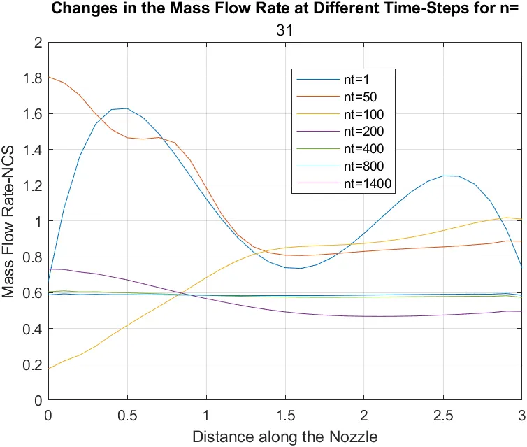
In the plot above, we can see how the mass flow rate changes with certain values of the time loop counter. Here, we can see that as the Time loop progresses, the system tries to achieve convergence and gets closer to the actual value of the mass flow rate for the system. The peak value out of all the time steps is achieved at time step number 50 where the Non-Dimensionalised Mass flow rate goes to around 2.1.
2. Change in the Primitive Variables with respect to time for the Non-Conservation Form.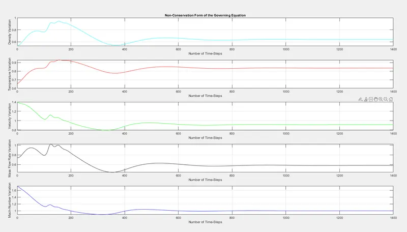
In the above plot, we can see how the primitive variables are varying with the different time-steps. As we can see that after about 700th time-step, there is no visible change in the variables. The Gradient has reduced and the system is reaching convergence.
3. Steady State Distribution of the Primitive Variables in the Nozzle: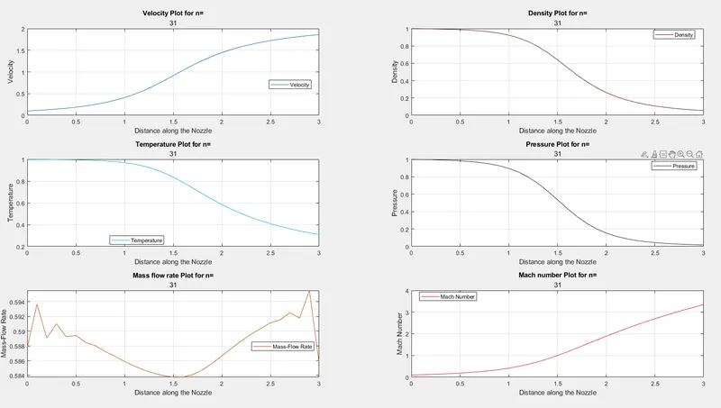
Here, we can see how the variables are changing in the Nozzle for the Non-conservation Form when the Seady State has been achieved. As, we can see that, both density and Temperature decrease whereas the Velocity and Mach number keeps on increasing as the flow is going from the Sub-sonic region to the Super-sonic region. Because the flow is in the super-sonic region, the velocity is bound to increase in that region.
4. Change in Mass-flow for the Conservation form.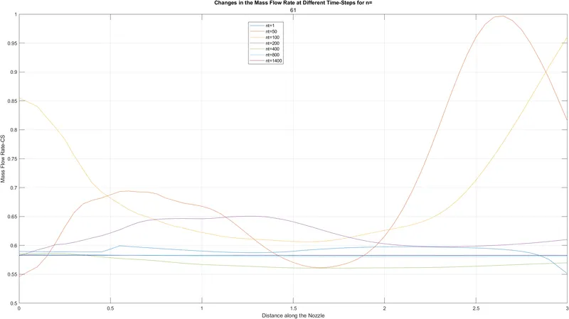
In the plot above, we can see how the mass flow rate changes with certain values of the time loop counter. Here, we can see that as the Time loop progresses, the system tries to achieve convergence and gets closer to the actual value of the mass flow rate for the system. The peak value out of all the time steps is achieved at time step number 50 where the Non-Dimensionalised Mass flow rate goes to around 1, this value is approximately half the peak that we achieved in the Non-Conservation Form of the Governing Equation.
5. Change in the Primitive Variables with respect to time for the Conservation Form.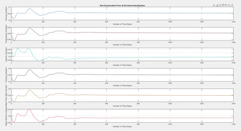
In the above plot, we can see how the primitive variables are varying with the different time-steps. As we can see that after about 700th time-step, there is no visible change in the variables. The Gradient has reduced and the system is reaching convergence.
6. Steady State Distribution of the Primitive Variables in the Nozzle for the Conservation Form.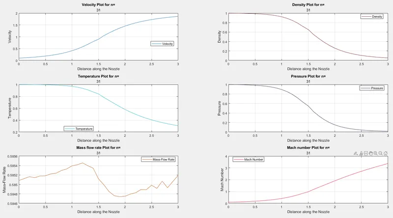
Here, we can see how the variables are changing in the Nozzle for the Non-conservation Form when the Seady State has been achieved. As, we can see that, both density and Temperature decrease whereas the Velocity and Mach number keeps on increasing as the flow is going from the Sub-sonic region to the Super-sonic region. Because the flow is in the super-sonic region, the velocity is bound to increase there.
7.Comparison in the flow rates between the Conservation and the Non-Conservation Form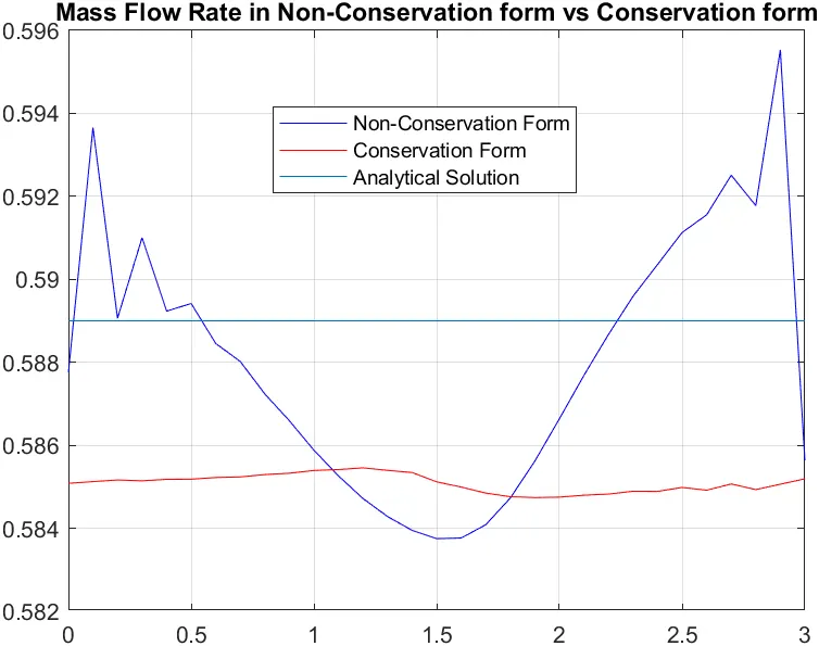
Here, we can clearly see that the conservation form does a better job of preserving mass throughout the flow field, mainly because the mass flow itself is one of the dependent variables in the equation and hence the mass flow is a primary result from the Conservation form of the Governing Equations.
Whereas, the dependent variables in the Non-Conservation form of the equations are the primitive variables and mass flow is obtained as a secondary result.
9. Grid Dependency Test:
The solution is said to be Grid Independent if the solutions have no effect on the number of grid points once the solution reaches a steady state. Let us double the number of grid points to 61 and then study the results.
We have run the same code as above and since I have already automated the time-step calculation and the calculation of the Throat properties according to the number of grid points, there is no need to change anything else in the main code, other than the number of grid points. The results are as follows:
a.Change in Mass-flow rate for the Non-conservation form.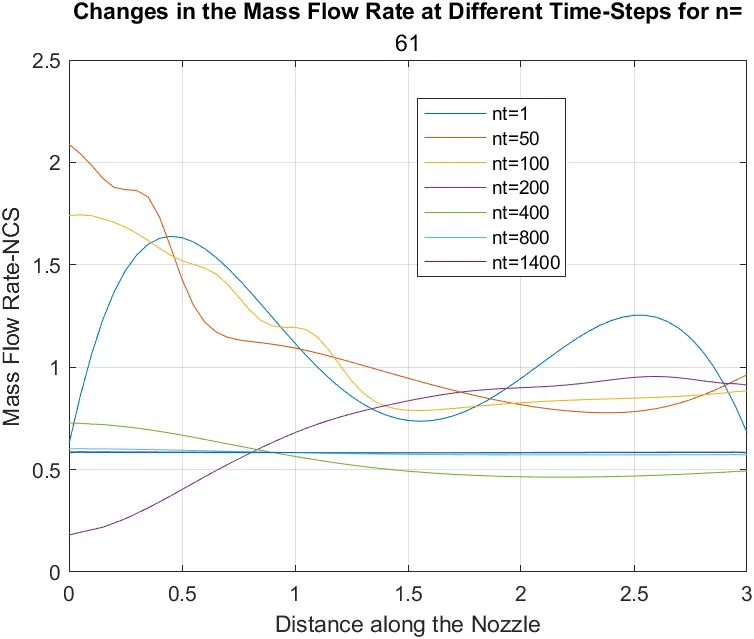
b.Change in the Primitive Variables with respect to time for the Non-Conservation Form.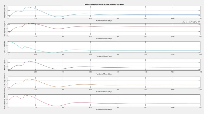
c.Steady State Distribution of the Primitive Variables in the Nozzle: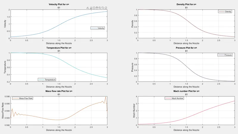
d. Change in Mass-flow rate for the Conservation form.
e.Change in the Primitive Variables with respect to time for the Conservation Form.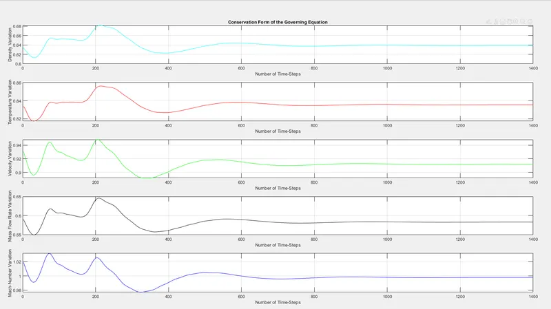
f. Steady State Distribution of the Primitive Variables in the Nozzle for the Conservation Form.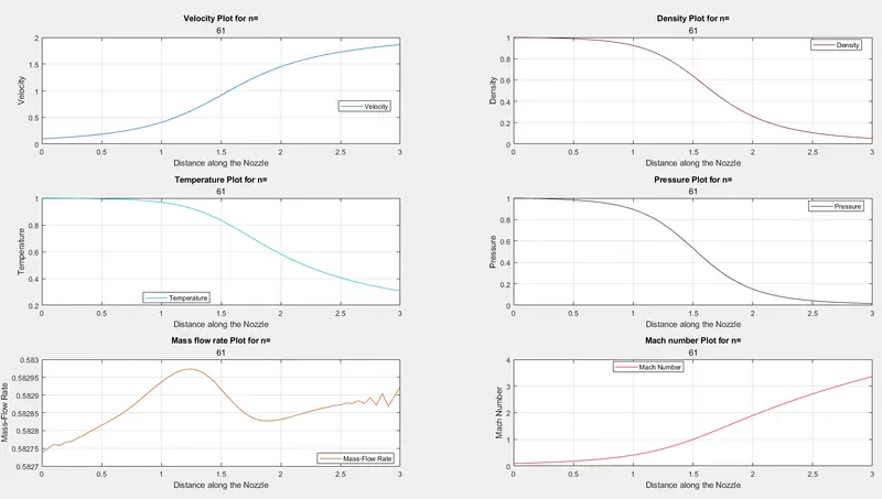
g.Comparison in the flow rates between the Conservation and the Non-Conservation Form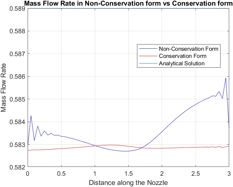
As we can see that, there is no considerable difference between the plots where the number of grid points is 31 and when we change the number of grid points to 61. The degree of Difference is relatively less(<5%), hence, we can conclude that the Solution is Grid independent.
The increase in the number of grid points will increase the simulation time and because there is no considerable change in the results as well. So, its better if we just simulate with the grid points equal to 31 instead of it being equal to 61. - Conclusions: In conclusion, I would like to state that this project helped me understand the 1D-Supersonic Nozzle flow in much better depth. Also, it helped me comprehend the MacCormack method as well. The following conclusions can be drawn between the Non-Conservation and the Conservation form of the Governing equation:
1. The Conservation Form gives a better Mass Flow Distribution because of the difference in the dependent and the independent variables of the two forms.
2. The Non-conservation form yeilds to much smaller Residuals.
3. As we understand that there is no clear difference between the two forms of the equation in terms of the accuracy of theResults that they yeild. The Non-conservation form yeilds gives a higher accuracy for primitive variables and the Conservation form of the Governing Equations will give a higher accuracy for the Flux variables.
4. When we wish to understand in terms of scripting the two forms, the Conservation Form requires a slightly more amount of work than when we script for the Non-Conservation form. This is because we need to decode the Primitive variables from the Flux Variables that we give in.