Week 7 - Simulation of a 1D Super-sonic nozzle flow simulation using Macormack Method
OBJECTIVE:
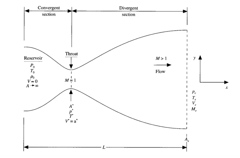
To simulate the isentropic flow through a quasi 1D subsonic-supersonic nozzle and derive both the conservation and non-conservation forms of the governing equations and sovle them using the MacCormack's technique.
Assumptions Made:
1. The flow is steady, isentropic through a convergent-divergent nozzle
2. The flow at the inlet comes from a reservoir where the pressure and temperature are denoted by p0 and T0, respectively.
3. The cross sectional area is theoricitically infinte`( A to infty)` and hence the velocity is very small `( V to 0)`
4. The flow expands isentropically to supersonic speeds at the nozzle exit.
5. The flow is locally subsonic in the convergent section of the nozzle, sonic at the throat and supersonic at the divergent section.
6. The time step calculation will be done using the CFL criterion .
Non Dimensional forms of Governing Equations
Non-Conservative form
Continuity equation
`(delrho')/(delt') = -rho' (delV')/(delx') - rho' V' (del(ln A'))/(delx') - V' (delrho')/(delx')`
Momentum Equation
`(delV')/(delt') = -V'(delV')/(delx') - (1/gamma)((delT')/(delx') +(T')/(p') (delrho')/(delx'))`
Energy Equation
`(delT')/(delt') = - V (delT')/(delx') - (gamma-1) T'[ (delV')/(delx') + V'((del(ln A'))/(delx'))]`
Conservative form
Continuity equation
`(delrho'A')/(delt') + (delrho'A'V')/(delx')`
Momentum Equation
`(delrho'A'V')/(delt') + (del[rho'A'V'^2 + (1/gamma) p'A'])/delx' = (1/gamma) p' (delA')/(delx')`
Energy Equation
`(del[rho'(((e')/(gamma-1)) + (gamma/2) V'^2 ) A'])/(delt') + (del[rho'(((e')/(gamma-1)) + (gamma/2) V'^2 ) V'A' + p'A'V']) / (delx') = 0`
Solution Vector
`U1 = rho'A'`
`U2 = rho'A'V'`
`U3 = rho'((e')/(gamma-1)+ (gamma/2) V'^2 ) A'`
Flux terms
`F1 = rho'A'V'`
`F2 = rho'A'V' + (1/gamma) p'A'`
`F3 = rho'((e')/(gamma-1)+ (gamma/2) V'^2 )V' A' + rho'A'V'`
Source term
`J2 = -(1/gamma) p' (delA')/(delx')`
Thus the Governing equations can be written as ,
`(delU1)/(delt') = -(delF1)/(delx')`
`(delU2)/(delt') = -(delF2)/(delx') + J2`
`(delU3)/(delt') = -(delF3)/(delx')`
Solving Technique
For solving this problem we are using the MacCormack technique. The governing equation will be in terms of partial differential equations suitable for time marching solution of quasi-one dimensional flow. The finite difference expressions pertaining to MacCormack's technique will be formulated .
Assumed data :
1. Number of grid points (n) = 31
2. gamma = 1.4
3. Courant number = 0.5
4. number of time steps = 1400
Main program
clear all
close all
clc

% inputs
n = 31;
x = linspace(0,3,n);
dx = x(2)-x(1);
gamma =1.4;
cfl = 0.5;
nt = 1:1400;
% Area
a = 1+(2.2*((x -1.5).^2));

% Calculating throat point
throat = ((n-1)/2)+1;

% Solving for conservative and non- conservative forms equation
tic
[rho,t,v,p,M,m,rho_throat,t_throat,v_throat,p_throat,M_throat,m_throat] = non_conservative(n,x,dx,gamma,cfl,nt,a,throat);
Time_non_conservative = toc;
fprintf('Time taken to solve non-conservative %4.2f secs \n',Time_non_conservative);

tic
[rho_c,t_c,v_c,p_c,M_c,m_c,rho_throat_c,t_throat_c,v_throat_c,p_throat_c,M_throat_c,m_throat_c] = Nozzle_flow_conservative(n,x,dx,gamma,cfl,nt,a,throat);
Time_conservative = toc;
fprintf('Time taken to solve conservative %4.2f secs',Time_conservative);

   %plotting
   figure(3)
   subplot(2,3,1)
   plot(nt,rho_throat,'r',nt,rho_throat_c,'b')
   xlabel('Time')
   ylabel('Non-Dimensional density')
   title('Variation of density at nozzle throat')
   legend('Non-Conservative','Conservative')
   subplot(2,3,2)
   plot(nt,v_throat,'r',nt,v_throat_c,'b')
   xlabel('Time')
   ylabel('Non dimensional velocity')
   title('Variation of velocity at nozzle throat')
   legend('Non-Conservative','Conservative')
   subplot(2,3,3)
   plot(nt,t_throat,'r',nt,t_throat_c,'b')
   xlabel('Time')
   ylabel('Non dimensional Temperature')
   title('Variation of Temperature at nozzle throat')
   legend('Non-Conservative','Conservative')
   subplot(2,3,4)
   plot(nt,p_throat,'r',nt,p_throat_c,'b')
   xlabel('Time')
   ylabel('Non dimensional pressure')
   title('Variation of Pressure at nozzle throat')
   legend('Non-Conservative','Conservative')
   subplot(2,3,5)
   plot(nt,M_throat,'r',nt,M_throat_c,'b')
   xlabel('Time')
   ylabel('Mach number ')
   title('Variation of Mach number at nozzle throat')
   legend('Non-Conservative','Conservative')
   subplot(2,3,6)
   plot(nt,m_throat,'r',nt,m_throat_c,'b')
   xlabel('Time')
   ylabel('Non dimensional mass flow rate')
   title('Variation of Mass flow rate at nozzle throat')
   legend('Non-Conservative','Conservative')

   figure(4)
   subplot(2,3,1)
   plot(x,rho,'r',x,rho_c,'b*')
   xlabel('Length of the nozzle')
   ylabel('Non-Dimensional density')
   title('Density profile')
   legend('Non-Conservative','Conservative')
   subplot(2,3,2)
   plot(x,v,'r',x,v_c,'b*')
   xlabel('Length of the nozzle')
   ylabel('Non dimensional velocity')
   title('Velocity profile')
   legend('Non-Conservative','Conservative')
   subplot(2,3,3)
   plot(x,t,'r',x,t_c,'b*')
   xlabel('Length of the nozzle')
   ylabel('Non dimensional Temperature')
   title('Temperature profile')
   legend('Non-Conservative','Conservative')
   subplot(2,3,4)
   plot(x,p,'r',x,p_c,'b*')
   xlabel('Length of the nozzle')
   ylabel('Non dimensional pressure')
   title('Pressure profile')
   legend('Non-Conservative','Conservative')
   subplot(2,3,5)
   plot(x,M,'r',x,M_c,'b*')
   xlabel('Length of the nozzle')
   ylabel('Mach number ')
   title('Mach number profile')
   legend('Non-Conservative','Conservative')
   subplot(2,3,6)
   plot(x,m,'r',x,m_c,'b*')
   xlabel('Length of the nozzle')
   ylabel('Non dimensional mass flow rate')
   title('Mass flow rate profile')
   legend('Non-Conservative','Conservative')
Non-conservative function
function [rho,t,v,p,M,m,rho_throat,t_throat,v_throat,p_throat,M_throat,m_throat] = non_conservative(n,x,dx,gamma,cfl,nt,a,throat)

% calculate inital profiles
rho = 1 - (0.3146*x);
t = 1 - (0.2314*x);
v = (0.1+(1.09*x)).*(t.^0.5);

%Time step size
for z = 1:n
  c = sqrt(t(z));
  dt(z) = cfl*(dx/(c + v(z)));
end
dt = min(dt);

% outer time loop
for k = 1:length(nt)
    %old values;
    rho_old = rho;
    v_old = v;
    t_old = t;

    %predictor method
    for j =2:n-1
        dvdx = (v(j+1)-v(j))/dx;
        drhodx = (rho(j+1)-rho(j))/dx;
        dtdx = (t(j+1)-t(j))/dx;
        dlogadx = (log(a(j+1))-log(a(j)))/dx;
         %continuity equation
        drhodt_p(j) = -rho(j)*dvdx -rho(j)*v(j)*dlogadx -v(j)*drhodx;
        %Momentum equation
        dvdt_p(j) = -v(j)*dvdx - (1/gamma)*(dtdx + (t(j)/rho(j))*drhodx);
        % Energy  equation
        dtdt_p(j) = -v(j)*dtdx - (gamma-1)*t(j)*(dvdx + v(j)*(dlogadx));
         % Solution update
         rho(j) = rho(j)+drhodt_p(j)*dt;
         v(j) = v(j)+dvdt_p(j)*dt;
         t(j) = t(j)+dtdt_p(j)*dt;

    end
    %Corrected method
    for j =2:n-1
        dvdx = (v(j)-v(j-1))/dx;
        drhodx = (rho(j)-rho(j-1))/dx;
        dtdx = (t(j)-t(j-1))/dx;
        dlogadx = (log(a(j))-log(a(j-1)))/dx;
         %continuity equation
        drhodt_c(j) = -rho(j)*dvdx -rho(j)*v(j)*dlogadx -v(j)*drhodx;
        %Momentum equation
        dvdt_c(j) = -v(j)*dvdx - (1/gamma)*(dtdx + (t(j)/rho(j))*drhodx);
        % Energy  equation
        dtdt_c(j) = -v(j)*dtdx - (gamma-1)*t(j)*(dvdx + v(j)*(dlogadx));
    end

    % Compute average time derivative

    drhodt  = 0.5*(drhodt_p + drhodt_c);
    dvdt  = 0.5*(dvdt_p + dvdt_c);
    dtdt = 0.5*(dtdt_p + dtdt_c);

    % Final solution update
      for i = 2:n-1
         rho(i) = rho_old(i)+drhodt(i)*dt;
         v(i) = v_old(i)+dvdt(i)*dt;
         t(i) = t_old(i)+dtdt(i)*dt;
      end

    % Boundary condition
    % Inlet
    v(1) = 2*v(2) - v(3);
    % Outlet;
    v(n) = 2*v(n-1) - v(n-2);
    rho(n) = 2*rho(n-1) - rho(n-2);
    t(n) = 2*t(n-1) - t(n-2);

      % calculating primitive variables  pressure and mach number
      for q = 1:n
         p(q) = rho(q) * t(q);
         M(q) = v(q) / (sqrt(t(q)));
      end

    % calculating the mass flow rate
    m = rho .* v.* a;


    % Capturing the values at the Throat section
    rho_throat(k) = rho(throat);
    v_throat(k) = v(throat);
    p_throat(k) = p(throat);
    t_throat(k) = t(throat);
    M_throat(k) = M(throat);
    m_throat(k) = m(throat);


    % mass flow rate plot
    figure(1)
    if  k==1
        plot (x,m,'b')
        hold on
    elseif k ==50
        plot (x,m,'r')
        hold on
    elseif k==100
        plot (x,m,'y')
        hold on
    elseif k==150
        plot (x,m,'g')
        hold on
    elseif k==200
        plot (x,m,'c')
        hold  on
    elseif k ==700
        plot (x,m,'magenta')
    legend ('1st time step' , '50th time step' , '100th time step' , '150th time step' , '200th time step' , '700th time step');
    xlabel('Nondimensional distance through the nozzle(x)');
    ylabel('Nondimensional mass flow rate');
    title('Variation of Mass flow rate distribution inside the nozzle at different time steps(NON-CONSERVATIVE)','FontSize',11);
    end


end
end
Conservative function
  function [rho,T,v,p,M,m,rho_throat,T_throat,v_throat,p_throat,M_throat,m_throat] = Nozzle_flow_conservative(n,x,dx,gamma,cfl,nt,a,throat)


%calculate intial profiles
for i = 1:length(x)
if x(i)<=0.5
    rho(i) = 1;
    T(i) = 1;
elseif x(i) > 0.5 && x(i)<=1.5
    rho(i) = 1 -0.366*(x(i)-0.5);
    T(i) = 1 - 0.167*(x(i)-0.5);
elseif x(i) >1.5 && x(i) <=3.5
    rho(i) = 0.634 - 0.3879*(x(i)-1.5);
    T(i) = 0.833 - 0.3507 *(x(i) -1.5);
end
end
% solution vectors
v = 0.59./(rho.*a);
u1 = rho.*a;
u2 = rho.*a.*v;
u3 = u1.*((T./(gamma-1))+(gamma/2).*(v.^2));

% calculating time step size
for z = 1:n
  c = sqrt(T(z));
  dt(z) = cfl*(dx/(c + v(z)));
end
dt = min(dt);

%Outer loop
for k = 1:length(nt)

    u1_old = u1;
    u2_old = u2;
    u3_old = u3;

    % flux vectors
    f1 = u2;
    f2 = (u2.^2./u1) + ((gamma-1)/gamma)*(u3 - ((gamma/2)*(u2.^2./u1)));
    f3 = (gamma*((u2.*u3)./u1)) - ((gamma*(gamma-1))/2)* ((u2.^3)./(u1.^2));

    %predictor step

    for j = 2:n-1
            dadx(j) = ((a(j+1))-(a(j)))/dx;
        % source term
        J2_p(j) =  (1/gamma)*(rho(j)*T(j))* dadx(j);

        %continuity eq
        du1dt_p(j) = -((f1(j+1) - f1(j))/dx);

        % Momentum eq
        du2dt_p(j) = - ((f2(j+1) - f2(j))/dx) +J2_p(j);

        % energy eq
        du3dt_p(j) = - ((f3(j+1) - f3(j))/dx) ;

        % Solution update
        u1(j) = u1(j) + du1dt_p(j) *dt;
        u2(j) = u2(j) + du2dt_p(j) *dt;
        u3(j) = u3(j) + du3dt_p(j) *dt;
    end

%     updating flux vectors
    f1 = u2;
    f2 = (u2.^2./u1) + ((gamma-1)/gamma)*(u3 - ((gamma/2)*(u2.^2./u1)));
    f3 = (gamma*((u2.*u3)./u1)) - ((gamma*(gamma-1))/2)* ((u2.^3)./(u1.^2));

    %  Corrected method
    for i = 2:n-1
            dadx(i)  = ((a(i))-(a(i-1)))/dx;
        %source term
        J2(i) =  (1/gamma)*(rho(i)*T(i))* dadx(i);
        %continuity eq
        du1dt_c(i) = -((f1(i) - f1(i-1))/dx);
        % Momentum eq
        du2dt_c(i) = - ((f2(i) - f2(i-1))/dx) +J2(i);
        % energy eq
        du3dt_c(i) = - ((f3(i) - f3(i-1))/dx) ;
    end

    % Compute average time derivative
      du1dt = 0.5*(du1dt_p + du1dt_c);
      du2dt = 0.5*(du2dt_p + du2dt_c);
      du3dt = 0.5*(du3dt_p + du3dt_c);

      % Final solution update
      for i = 2:n-1
            u1(i) = u1_old(i) + du1dt(i)*dt;
            u2(i) = u2_old(i) + du2dt(i)*dt;
            u3(i) = u3_old(i) + du3dt(i)*dt;
      end

       % Boundary condition
       %inlet
       u1(1) = rho(1)*a(1);
       u2(1) = 2*u2(2) - u2(3);
       u3(1) = u1(1)*( (T(1)/(gamma-1)) + (gamma/2)* (v(1).^2));

       %outlet
       u1(n) = 2*u1(n-1) - u1(n-2);
       u2(n) = 2*u2(n-1) - u2(n-2);
       u3(n) = 2*u3(n-1) - u3(n-2);

       % updating the primitive values
       rho = u1./a;
       v = u2./u1;
       T = (gamma-1)* ((u3./u1) - (gamma/2)*(v.^2));

      % calculating primitive variables  pressure and mach number
      for q = 1:n
         p(q) = rho(q) * T(q);
         M(q) = v(q) / (sqrt(T(q)));
      end

    % calculating the mass flow rate
    m = rho .* v.* a;

    % Capturing the values at the Throat section
    rho_throat(k) = rho(throat);
    v_throat(k) = v(throat);
    p_throat(k) = p(throat);
    T_throat(k) = T(throat);
    M_throat(k) = M(throat);
    m_throat(k) = m(throat);


    % mass flow rate plot
    figure(2)
    if  k==1
        plot (x,m,'b')
        hold on
    elseif k ==50
        plot (x,m,'r')
        hold on
    elseif k==100
        plot (x,m,'y')
        hold on
    elseif k==150
        plot (x,m,'g')
        hold on
    elseif k==200
        plot (x,m,'c')
        hold  on
    elseif k ==700
        plot (x,m,'magenta')
    legend ('1st time step' , '50th time step' , '100th time step' , '150th time step' , '200th time step' , '700th time step');
    xlabel('Nondimensional distance through the nozzle(x)');
    ylabel('Nondimensional mass flow rate');
    title('Variation of Mass flow rate distribution inside the nozzle at different time steps(CONSERVATIVE)','FontSize',11);
    end

end
end
Output:
Steady-state distribution of primitive variables inside the nozzle
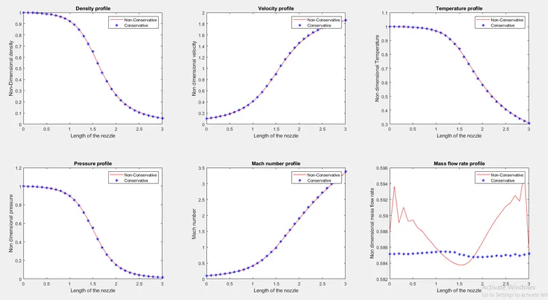
In the case of Mass flow rate distribution .The Non conservation results have severe oscillations at both inflow and outflow boundaries.The conservation form does a better job of preserving mass throughout the flow field because the mass flow itself is one of the dependent variables in the equations
Time-wise variation of the primitive variables
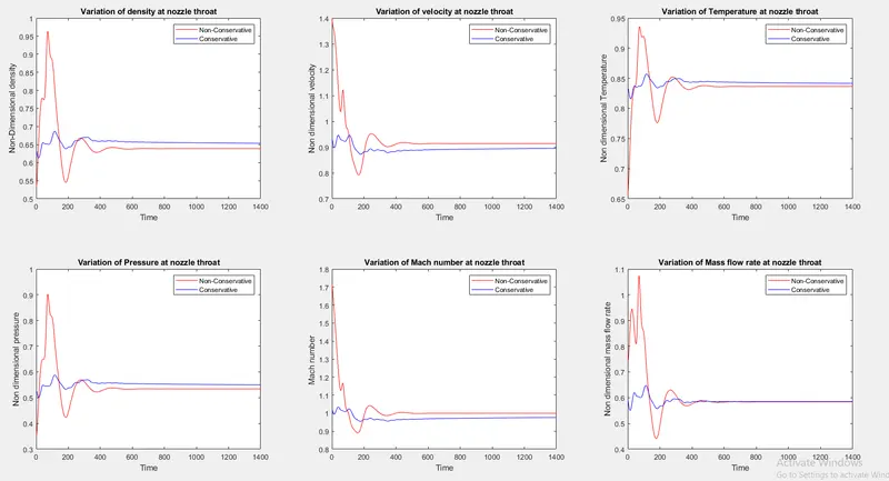
The largest variations occur at early time steps this is because the flow field variables are driven by stronger potential and hence they change rapidly as time progresses the variations are smaller as it eases towards steady state
Comparison of Normalized mass flow rate distributions of both forms
Non Conservative:
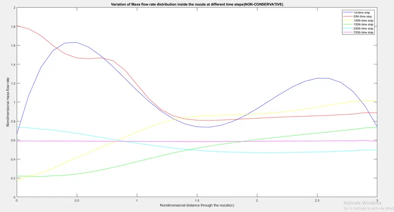
Conservative :
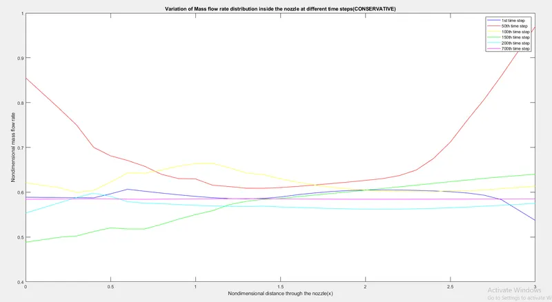
The Non-dimensional mass flow rate versus nozzle length (Figure 4) The results shows that after time step 1 the mass flow rate deviates from the inital condition After 200 time steps the mass flow rate is becoming more stable and after 700 time steps it is almost equal to a constant value, comparing the reults obtained using Non conservative form(Figure3) the variation in mass flow are less severe in case of Conservative form
Grid Independence Results:
Grid independence test is done for 3 different grid points n = 31,61,91 respectively
| `rho/rho0` | `T/T0` | `p/p0` | `M` | `m` | |
| Exact Analytical Solution | 0.634 | 0.833 | 0.528 | 1 | 0.579 |
| Conservative form (n=31) | 0.6535 | 0.8416 | 0.5500 |
0.9760 |
0.5851 |
| Conservative form (n=61) | 0.6392 | 0.8358 | 0.5343 | 0.9974 | 0.5829 |
| Conservative form (n=91) |
0.6375 |
0.8358 | 0.5328 | 0.9998 | 0.5827 |
| Non- Conservative form (n=31) | 0.6387 | 0.8365 | 0.5342 | 0.9994 | 0.5838 |
| Non-Conservative form (n=61) | 0.6377 | 0.8354 | 0.5327 | 0.9998 | 0.5827 |
| Non-Conservative form (n=91) | 0.6404 | 0.8368 | 0.5359 | 1.0026 | 0.5874 |
Excecution Time Comparison for both forms :
| n = 31 | n = 61 | n = 91 | |
| Excecution time for Non-conservative | 1.49 secs | 1.50 secs | 1.52 secs |
| Excecution time for Conservative | 0.77 secs | 0.78 secs | 0.79 secs |
Results and Observations :
1. The conservation form yields a better mass flow distribution thorught the flow field . It does a better job of conserving mass
2. The time taken to solve the conservative form is less compared to Non-conservative form . Also setting up the solution algorithm is more tedious in the case of conservative form as it invloves solving using the flux variables and then decoding the primitive variables. In the case of non- conservative form equations are solved using primitive variables itself.
3. The steady state results obtained from both forms of governing equation are essentially the same, with slight notable differences.
4. From the table above it is proven that the initial solution with n=31 (n - number of grid points ) is Grid Independent as there are no significant changes in the results.