Week 5 - Mid term project - Solving the steady and unsteady 2D heat conduction problem
The 2D conduction equation
`(delT)/(delt) = alpha((del^2T)/(delx^2) + (del^2T)/(dely^2))`
where `alpha` is the thermal diffusivity of material
In Steady state flow the temperature does not change with time. Therefore the time derivative term is neglected
`((del^2T)/(delx^2) + (del^2T)/(dely^2)) = 0`
The following assumptions are made
1. Assume a domain is a unit square
2. Assume nx = 10 =ny
3. Boundary conditions
1. Left = 400K
2. right = 800K
3. Bottom = 900K
4. Top = 600K
4. Tolerance = 1e-4
5. Error = 9e9
6. Thermal diffusivity = 1.4
7. omega = 1.4
Solving the steady state equation
`((del^2T)/(delx^2) + (del^2T)/(dely^2)) = 0`
The discretised equation is
`T(i,j) = 1/k{((Told(i-1,j)+Told(i+1,j))/dx^2) + ((Told(i,j-1)+Told(i,j+1))/dy^2)}`
`k = 2((dx^2 +dy^2)/(dx^2 *dy^2))`
Function code for jacobi
function T = jacobi_iter(T,dx,dy,nx,ny,k,Told,error,tol,X,Y)

jacobi_iter = 1;
while(error > tol)
    for i = 2:nx-1
        for j =2:ny-1
            term1 = (Told(i-1,j)+Told(i+1,j))/(k*(dx^2));
            term2 = (Told(i,j-1)+Told(i,j+1))/(k*(dy^2));
            T(i,j) = term1+ term2;
        end
    end
    error = max(max(abs(Told - T)));
    Told  = T;
    jacobi_iter = jacobi_iter + 1;
    figure(1)
    [c,d] = contourf(X,Y,T);
    colormap = (jet)
    colorbar
    clabel(c,d)
    xlabel('x axis');
    ylabel('y axis');
    set (gca,'ydir','reverse');
    title_text = sprintf('Iteration number = %d',jacobi_iter);
    title(title_text);
    pause(0.03);
end
end
Function code for Gauss seidel
function T = GS_iter(T,dx,dy,nx,ny,k,Told,error,tol,X,Y)

GS_iter = 1;
while(error > tol)
    for i = 2:nx-1
        for j =2:ny-1
            term1 = (T(i-1,j)+Told(i+1,j))/(k*(dx^2));
            term2 = (T(i,j-1)+Told(i,j+1))/(k*(dy^2));
            T(i,j) = term1+ term2;
        end
    end
    error = max(max(abs(Told - T)));
    Told  = T;
    GS_iter = GS_iter + 1;
    figure(2)
    [c,d] = contourf(X,Y,T);
    colormap = (jet)
    colorbar
    clabel(c,d)
    xlabel('x axis');
    ylabel('y axis');
    set (gca,'ydir','reverse');
    title_text = sprintf('Iteration number = %d',GS_iter);
    title(title_text);
    pause(0.03);
end
end
Function code for SOR
function T = sor_iter(T,dx,dy,nx,ny,k,Told,error,tol,X,Y)

sor_iter = 1;
omega = 1.4;
while(error > tol)
    for i = 2:nx-1
        for j =2:ny-1
            term1 = (T(i-1,j)+Told(i+1,j))/(k*(dx^2));
            term2 = (T(i,j-1)+Told(i,j+1))/(k*(dy^2));
            T_GS = term1+ term2;
            T(i,j) = (1-omega)*(Told(i,j)) + omega*(T_GS);
        end
    end
    error = max(max(abs(Told - T)));
    Told  = T;
    sor_iter = sor_iter + 1;
    figure(3)
    [c,d] = contourf(X,Y,T);
    colormap = (jet)
    colorbar
    clabel(c,d)
    xlabel('x axis');
    ylabel('y axis');
    set (gca,'ydir','reverse');
    title_text = sprintf('Iteration number = %d',sor_iter);
    title(title_text);
    pause(0.03);
end
end
Main code
clear all
close all
clc

%Defining the inputs
nx = 10;
ny = 10;
x = linspace(0,1,nx);
y = linspace(0,1,ny);
dx = x(2) - x(1);
dy = y(2) - y(1);
[X,Y] = meshgrid(x,y);

%Defining the BC
T = ones(nx,ny);
T(1,:) = 600;
T(10,:) = 900;
T(:,10) = 800;
T(:,1) = 400;

T(1,1) = 500;
T(1,10) = 700;
T(10,1) = 650;
T(10,10) = 850;

%Initial condition
Told = T;
error = 9e9;
tol = 1e-4;
k = 2*((dx^2+dy^2)/(dx^2*dy^2));

%Calling the different solvers
iterative_solver = input('Enter the solver to be used');
if iterative_solver ==1
    tic;
    T_jacobi = jacobi_iter(T,dx,dy,nx,ny,k,Told,error,tol,X,Y);
    Time_jacobi = toc
elseif iterative_solver ==2
    tic;
    T_Gauss = GS_iter(T,dx,dy,nx,ny,k,Told,error,tol,X,Y);
    Time_GS = toc
elseif iterative_solver ==3
     tic;
    T_SOR = sor_iter(T,dx,dy,nx,ny,k,Told,error,tol,X,Y);
    Time_SOR = toc
end
Results
Jacobi
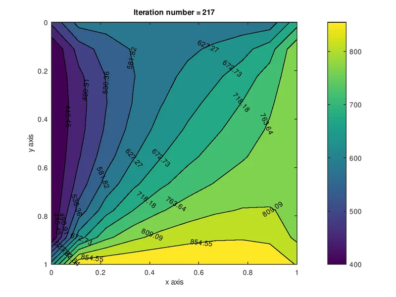
Time_jacobi = 86.305
Gauss Seidel
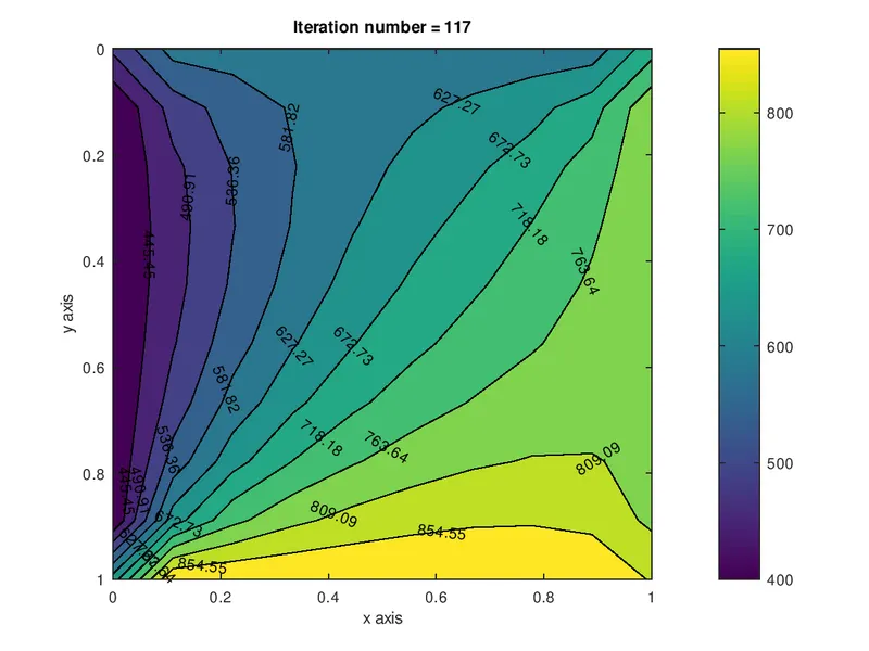
Time_GS = 46.553
SOR
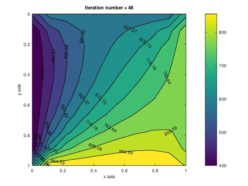
Time_SOR = 19.304
Disccusions
From the plots we can see that the SOR takes less computational time and less iterations compared with other methods.
Solving the Transient equation
`(delT)/(delt) = alpha((del^2T)/(delx^2) + (del^2T)/(dely^2))`
Solving the equation explicitly
In this method, each equation has only one unknown and can be solved explicitly
The discretized equation is
`T(i,j) = T^n + k1(T^nold(i+1,j) - 2T^nold(i,j) + T^nold(i-1,j) +k2(T^nold(i,j-1) - 2T^nold(i,j) + T^nold(i,j+1))`
`k1 = 2(alpha*dt/(dx^2))`
`k1 = 2(alpha*dt/(dy^2))`
Function code
function T = jacobi_iter_transient(T,dx,dy,nx,ny,k1,k2,Told,error,tol,X,Y)

jacobi_iter = 1;
    for k = 1:1400
        while(error>tol)
    for i = 2:nx-1
        for j =2:ny-1
            term1 = Told(i,j);
            term2 = k1*(Told(i-1,j)- 2*(Told(i,j))+Told(i+1,j));
            term3 = k2*(Told(i,j-1)-2*(Told(i,j))+Told(i,j+1));
            T(i,j) = term1+ term2+ term3;
        end
    end
    error = max(max(abs(T-Told)));
     jacobi_iter = jacobi_iter + 1;
    Told  = T;
    figure(1)
    [c,d] = contourf(X,Y,T);
    colormap = (jet)
    colorbar
    clabel(c,d)
    xlabel('x axis');
    ylabel('y axis');
    set (gca,'ydir','reverse');
    title_text = sprintf('Iteration number = %d',jacobi_iter);
    title(title_text);
    pause(0.03)
        end
    end
end
Main code
clear all
close all
clc

%Defining the inputs
nx = 10;
ny = 10;
x = linspace(0,1,nx);
y = linspace(0,1,ny);
dx = x(2) - x(1);
dy = y(2) - y(1);
dt = 0.01;
[X,Y] = meshgrid(x,y);
alpha = 1e-1;

%Defining the BC
T = ones(nx,ny);
T(1,:) = 600;
T(10,:) = 900;
T(:,10) = 800;
T(:,1) = 400;

%Initial condition
Told = T;
error = 9e9;
tol = 1e-4;
k1 = alpha*(dt/(dx^2));
k2 = alpha*(dt/(dy^2));

%solver
tic;
T_jacobi = jacobi_iter_transient(T,dx,dy,nx,ny,k1,k2,Told,error,tol,X,Y)
Time_jacobi = toc
Results
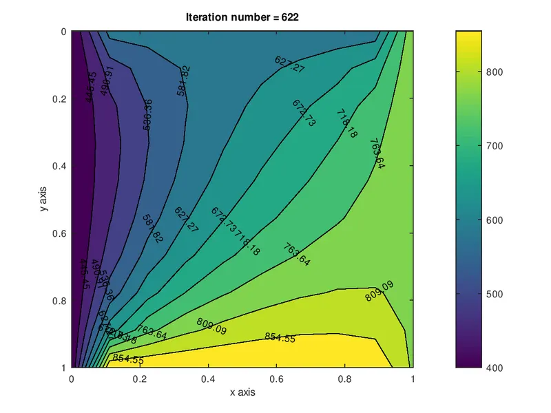
Time_jacobi = 249.42
Solving the above equation implicitly
The discretized equation is
`T(i,j) = (1/(1+2k1+2k2))[T^n + k1((T^nold(i+1,j) - 2T^nold(i,j) + T^nold(i-1,j))^(n+1)] +k2(T^nold(i,j-1) - 2T^nold(i,j) + T^nold(i,j+1)))^(n+1)`
`k1 = 2(alpha*dt/(dx^2))`
`k1 = 2(alpha*dt/(dy^2))`
Results
Jacobi
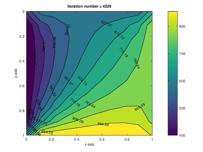
Time_jacobi = 554.39
Gauss seidel
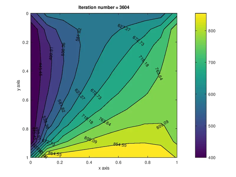
Time_GS = 551.16
SOR
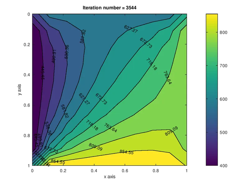
Time_SOR = 539.46
Disccusions
From the results we can see that no of iterations required and time taken for solving the equations decreases from jacobi to GS to SOR methods
jacobi > Gauss seidel > SOR
Also the transient simulation takes more iterations and time as compared to steady state solution because the equation has to be solved at every timestep in case of unsteady state simulation
Also the unsteady state problem is solved much faster in case of explicit solution compared to implicit method