Week 3 - Taylor table method and Matlab code
Derivation of 4th order approximation of second order derivative
1. Central Difference apprx
`(del^2f)/(delx^2) = af(i-2) +bf(i-1)+cf(i)+df(i+1)+ef(i+2)`
| `f(i)` | `Deltaxf'(i)` | `Deltax^2f''(i)` | `Deltax^3f'''(i)` | `Deltax^4f''''(i)` | |
| `af(i-2)` | `a` | `-2a` | `(4a)/2` | `-(8a)/6` | `(16a)/24` |
| `bf(i-1)` | `b` | `-b` | `b/2` | `-b/6` | `b/24` |
| `cf(i)` | `c` | `0` | `0` | `0` | `0` |
| `df(i+1)` | `d` | `d` | `d/2` | `d/6` | `d/24` |
| `ef(i+2)` | `e` | `2e` | `(4e)/2` | `(8e)/6` | `(16a)/24` |
| `0` | `0` | `1` | `0` | `0` |
`[[1,1,1,1,1],[-2,-1,0,1,2],[4/2,1/2,0,1/2,4/2],[-8/6,-1/6,0,1/6,8/6],[16/24,1/24,0,1/24,16/24]]` `[[a],[b],[c],[d],[e]]` = `[[0],[0],[1],[0],[0]]`
This is of the form AX = B with 5 unknowns and 5 equations.
Solving this in Matlab we get the coeffecients a b c d and e.
2. Skewed right-sided difference
`(del^2f)/(delx^2) = af(i)+bf(i+1)+cf(i+2)+df(i+3)+ef(i+4)+gf(i+5)`
| `f(i)` | `Deltaxf'(i)` | `Deltax^2f''(i)` | `Deltax^3f'''(i)` | `Deltax^4f''''(i)` | `Deltax^5f'''''(i)` | |
| `af(i)` | `a` | `0` | `0` | `0` | `0` | `0` |
| `bf(i+1)` | `b` | `b` | `b/2` | `b/6` | `b/24` | `b/120` |
| `cf(i+2)` | `c` | `2c` | `(4c)/2` | `(8c)/6` | `(16c)/24` | `(32c)/120` |
| `df(i+3)` | `d` | `3d` | `(9d)/2` | `(27d)/6` | `(81d)/24` | `(243d)/120` |
| `ef(i+4)` | `e` | `4e` | `(16e)/2` | `(64e)/6` | `(256e)/24` | `(1024e)/120` |
| `gf(i+5)` | `g` | `5e` | `(25g)/2` | `(125g)/6` | `(625g)/24` | `(3125g)/120` |
| `0` | `0` | `1` | `0` | 0 | 0 |
`[[1,1,1,1,1,1],[0,1,2,3,4,5],[0,1/2,2,9/2,16/2,25/2],[0,1/6,8/6,27/6,64/6,125/6],[0,1/24,16/24,81/24,256/24,625/24],[0,1/120,32/120,243/120,1024/120,3125/120]]``[[a],[b],[c],[d],[e],[g]]` = `[[0],[0],[1],[0],[0],[0]]`
This is of the form AX = B with 6 unknowns and 6 equations.
Solving this in Matlab we get the coeffecients a b c d e and g.
3. Skewed left-sided difference
`(del^2f)/(delx^2) = af(i-5) +bf(i-4)+cf(i-3)+df(i-2)+ef(i-1)+gf(i)`
| `f(i)` | `Deltaxf'(i)` | `Deltax^2f''(i)` | `Deltax^3f'''(i)` | `Deltax^4f''''(i)` | `Deltax^5f'''''(i)` | |
| `af(i-5)` | `a` | `-5a` | `(25a)/2` | `-(125a)/6` | `(625a)/24` | `-(3125a)/120` |
| `bf(i-4)` | `b` | `-4b` | `(16b)/2` | `-(64b)/6` | `(256b)/24` | `-(1024b)/120` |
| `cf(i-3)` | `c` | `-3c` | `(9c)/2` | `-(27c)/6` | `(81c)/24` | `-(243c)/120` |
| `df(i-2)` | `d` | `-2d` | `(4d)/2` | `-(8d)/6` | `(16d)/24` | `-(32d)/120` |
| `ef(i-1)` | `e` | `-e` | `e/2` | `-e/6` | `e/24` | `-e/120` |
| `gf(i)` | `g` | `0` | `0` | `0` | `0` | `0` |
| `0` | `0` | `1` | `0` | `0` | `0` |
`[[1,1,1,1,1,1],[-5,-4,-3,-2,-1,0],[25/2,16/2,9/2,4/2,1/2,0],[-125/6,-64/6,-27/6,-8/6,-1/6,0],[625/24,256/24,81/24,16/24,1/24,0],[-3125/120,-1024/120,-243/120,-32/120,-1/120,0]]` `[[a],[b],[c],[d],[e],[g]]` = `[[0] ,[0] ,[1] ,[0] ,[0], [0]]`
This is of the form AX = B with 6 unknowns and 6 equations.
Solving this in Matlab we get the coeffecients a b c d e and g.
Skewed Schemes
No of nodes = P+q = Order of derivative + order of approximation = 2+4
No of nodes taken for solving the scheme = 6
Hence proved that the skewed schemes are fourth order accurate
Advantage of Skewed Scheme
A skewed scheme is particularly useful where in solving flows involving only in one direction. Skewed schemes are uselful for capturing the physics at the boundaries wherein central difference schemes would require two points since there are no grid points available beyind the boundary .
Central differenence scheme
function out = central_difference_scheme(x,dx)

%analytical derivative
%function = exp(x) * cos(x)
analytical_derivative = -2*exp(x)*sin(x);

%Function defenition
f = @(x) exp(x)*cos(x);

%calculating the values of coeff;
syms a b c d e g ;
A  = [1 1 1 1 1;-2 -1 0 1 2;4/2 1/2 0 1/2 4/2;-8/6 -1/6 0 1/6 8/6 ;16/24 1/24 0 1/24 16/24];
B  = [ 0 ; 0; 1; 0;0;]
X = inv(A)*B;
a = X(1);
b = X(2);
c = X(3);
d = X(4);
e = X(5);

%numerical derivative
central_diff = (a*f(x-(2*dx))+b*f(x-dx)+c*f(x)+d*f(x+dx)+e*f(x+(2*dx)))/(dx^2);
out = abs(central_diff - analytical_derivative);

end
Right skewed scheme
function out = right_skewed_scheme(x,dx)

%analytical derivative
%function = exp(x) * cos(x)
analytical_derivative = -2*exp(x)*sin(x);

%Function defenition
f = @(x) exp(x)*cos(x);

%calculating the values of coeff;
syms a b c d e g ;
A  = [1 1 1 1 1 1 ; 0 1 2 3 4 5 ; 0 1/2 2 9/2 16/2 25/2 ;0 1/6 8/6 27/6 64/6 125/6 ; 0 1/24 16/24 81/24 256/24 625/24 ;0 1/120 32/120 243/120 1024/120 3125/120];
B = [0; 0; 1 ;0 ;0 ;0];
X = inv(A)*B ;

a = X(1);
b = X(2);
c = X(3);
d = X(4);
e = X(5);
g = X(6);

%numerical derivative
right_skewed = ((a*f(x)) + (b*f(x+dx)) + (c*(f(x+(2*dx)))) + (d*(f(x+(3*dx)))) + (e*f(x+(4*dx)))+ (g*f(x+(5*dx))))/(dx^2);
out = abs(right_skewed - analytical_derivative);

end
Left Skewed scheme
function out = left_skewed_scheme(x,dx)

%analytical derivative
%function = exp(x) * cos(x)
analytical_derivative = -2*exp(x)*sin(x);


%Function defenition
f = @(x) exp(x)*cos(x);

%calculating the values of coeff;
syms a b c d e g ;
A = [1 1 1 1 1 1 ; -5 -4 -3 -2 -1 0  ; 25/2 16/2 9/2 4/2 1/2 0 ; -125/6 -64/6 -27/6 -8/6 -1/6 0 ;625/24 256/24 81/24 16/24 1/24 0 ; -3125/120  1024/120  243/120 -32/120 -1/120 0];
B = [0 ;0 ;1 ;0 ;0 ;0];
X = inv(A)*B ;

a = X(1);
b = X(2);
c = X(3);
d = X(4);
e = X(5);
g = X(6);

%numerical derivative
left_skewed = (a*f(x-(5*dx)) + b*f(x-(4*dx)) + c*f(x-(3*dx)) + d*f(x-(2*dx)) + e*f(x-dx) + g*f(x))/(dx^2);
out = abs(left_skewed - analytical_derivative);

end
Main program
clear all
close all
clc

% input ;
x = pi/4;
dx = linspace(pi/40,pi/3,20);

%function = exp(x) * cos(x)
analytical_derivative = -2*exp(x)*sin(x);


for i = 1:length(dx)

  central_error(i) = central_difference_scheme(x,dx(i));
  right_skewed_error(i) = right_skewed_scheme(x,dx(i));
  left_skewed_error(i) = left_skewed_scheme(x,dx(i));

end

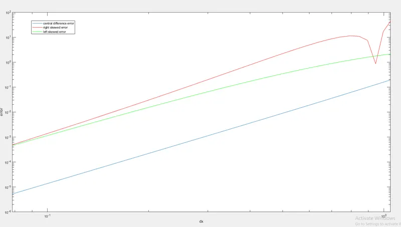
figure(1)
loglog(dx,central_error)
hold on
loglog(dx,right_skewed_error,'r')
hold on
loglog(dx,left_skewed_error,'g')

legend('central difference error', 'right skewed error','left skewed error')
xlabel('dx')
ylabel('error')
Output: