Week 7 - Simulation of a 1D Super-sonic nozzle flow simulation using Macormack Method
Simulation of a Quasi 1-D Supersonic nozzle flow simulation using Macormack Method
In this challenge, you are going to simulate the isentropic flow through a quasi 1D subsonic-supersonic nozzle. You will derive both the conservation and non-conservation forms of the governing equations and solve them using MacCormack's technique. You need to determine the steady-state temperature distribution for the flow-field variables and investigate the difference between the two forms of governing equations by comparing their solutions.
You need to show the following plots inside your report
1. Steady-state distribution of primitive variables inside the nozzle
2. Time-wise variation of the primitive variables
3. Variation of Mass flow rate distribution inside the nozzle at different time steps during the time-marching process
4. Comparison of Normalized mass flow rate distributions of both forms
Expected Results:
- Perform a grid independence test on the solution and explain all your findings.
- The code must be modular. You need to write separate functions to solve both forms.
- Discuss all the plots you are providing with observed inferences.
INTRODUCTION TO QUASI ONE-DIMENSIONAL ISENTROPIC NOZZLE FLOW:
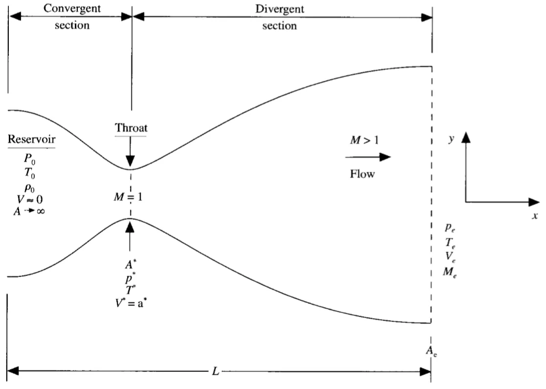
We consider the steady, isentropic flow through a convergent-divergent nozzle. The flow at the inlet to the nozzle comes from a reservoir where the pressure and temperature are denoted by `P_o`, and `T_o`, respectively. The cross-sectional area of the reservoir is large (theoretically, `A =>infty`), and hence the velocity is very small (`V =>0`). Thus,` P_o` and `T_o` are the stagnation values, or total pressure and total temperature, respectively. The flow expands isentropically to supersonic speeds at the nozzle exit, where the exit pressure, temperature, velocity, and Mach number are denoted by `P_e, T_e, V_e, and M_e,` respectively. The flow is locally subsonic in the convergent section of the nozzle, sonic at the throat (minimum area), and supersonic at the divergent section. The sonic flow (M = 1) at the throat means that the local velocity at this location is equal to the local speed of sound.
We assume that at a given section, where the cross-sectional area is A, the flow properties are uniform across that section. Hence, although the area of the nozzle changes as a function of distance along with the nozzle, `x`, and therefore in reality the flow field is two-dimensional (the flow varies in the two-dimensional `xy` space), we make the assumption that the flow properties vary only with x; this is tantamount to assuming uniform flow properties across any given cross-section. Such flow is defined as quasi-one-dimensional flow,
Governing equations unsteady Quasi-one-dimensional flow:
Continuity equation:
Conservative form : `(del(rho A))/(del t) + (del(rho A V))/(del x) = 0`
Non-Conservative form :`A (del rho)/(del t) + V (del(rho A))/(del x) = -rho A (del V)/(del x)`
Momentum equation:
Conservative form : `(del(rho A V))/(del t) + (del(rho A V^2))/(del x) = -A (del p)/(del x)`
Non-Conservative form : `rho (del V)/(del t) + rho V(del V)/(del x) = -(del p)/(del x)`
Energy equation:
Conservative form : `(del[rho (e + V^2/2) A])/(del t) + (del[rho (e + V^2/2) VA])/(del x) = - (del(p A V))/(del x)`
Non-Conservative form :`rho (del e)/(del t) + rho V(del e)/(del x) = - p(del V)/(del x) - pV(del(ln A))/(del x)`
Governing equations unsteady Quasi-one-dimensional flow in dimensional form:
| Conservative form : | Non-Conservative form : | |
| Continuity equation: | `(del(rho A))/(del t) + (del(rho A V))/(del x) = 0` | `A (del rho)/(del t) + V (del(rho A))/(del x) = -rho A (del V)/(del x)` |
| Momentum equation: | `(del(rho A V))/(del t) + (del(rho A V^2))/(del x) = -A (del p)/(del x)` | `rho (del V)/(del t) + rho V(del V)/(del x) = -(del p)/(del x)` |
| Energy equation: | `(del[rho (e + V^2/2) A])/(del t) + (del[rho (e + V^2/2) VA])/(del x) = - (del(p A V))/(del x)` | `rho (del e)/(del t) + rho V(del e)/(del x) = - p(del V)/(del x) - pV(del(ln A))/(del x)` |
The above equations are written in terms of dimensional variables. At this stage, we could readily proceed to set up our numerical solution for above equations. This is fine, and many CFD solutions are carried out directly in terms of such dimensional variables. Indeed, this has an added engineering advantage because it gives you a feeling for the magnitudes of the real physical quantities as the solution progresses. However, for nozzle flows, the flow-field variables are frequently expressed in terms of nondimensional variables, where the flow variables are referenced to their reservoir values. The nondimensional variables `P/P_o,rho/rho_o, & T/T_o`, vary between 0 and 1, which is an "aesthetic" advantage when presenting the results. Because fluid dynamicists dealing with nozzle flows so frequently use these nondimensional terms, we will follow suit here. (A number of CFD practitioners prefer to always deal with nondimensional variables, whereas others prefer dimensional variables; as far as the numerics are concerned, there should be no real difference, and the choice is really a matter of your personal preference). there for non dimensional flow variables are:-
| `T' = T/T^o` | `rho' = rho/rho^o` | `x' = x/L` | `V' = V/a_o` |
| `a_o = sqrt(gamma R T_o)` | `t'= t/(L/a_o)` | `A'= A/(A^**)` |
`L `= length of Nozzle
`L `= length of Nozzle
`T^o,rho^o` reservoir temperature and density
`a_o` = speed of sound in the reservoir
`A^**` = Sonic throat area
for perfect gas `e = C_vT` then the energy equation become
Governing equations unsteady Quasi-one-dimensional flow in Non-dimensional form:
| Conservative form : | Non-Conservative form : | |
| Continuity equation: | `(del(rho' A'))/(del t') + (del(rho' A' V'))/(del x') = 0` | `(del rho')/(del t') = -rho' (del V')/(del x') - rho' V' (del (ln A'))/(del x') - V'(del rho')/(del x')` |
| Momentum equation: | `(del(rho' A' V'))/(del t') + (del[rho' A' V'^2 + (1/gamma)p'A'])/(del x') = 1/gamma p' (del A')/(del x')` | `(del V')/(del t') = -V'(del V')/(del x') - 1/gamma((del T')/(del x') + (T')/(rho') (del rho')/(del x'))` |
| Energy equation: | `(del[rho'((e')/(gamma-1) + gamma/2 V'^2)A'])/(del t') + (del[rho'((e')/(gamma-1) + gamma/2 V'^2)V'A' + rho'A'V'])/(del x')` | `(del T')/(del t') = -V'(del T')/(del x') - (gamma-1)T'[(del V')/(del x') + V' (del(ln A'))/(del x')]` |
Numerical solutions for above non dimensional governing equations can be obtained by discretizing them. for this we are going to use MacCormack discretization technique. simply called as MacCormack technique.
MacCormack technique
MacCormack discretization technique is an explicit finite-difference technique to solve time marching PDEs and to obtain finite-difference solutions with second-order accuracy for both space and time derivatives.
MacCormack technique consists of three steps they are:-
- Predictor step:- in this predictor step we replace the spatial derivatives on the right-hand side with forward differences in the continuity equation, and to obtain predicted value we are going to use the first two terms of the Taylor series. the solution obtained in the step is only first-order accurate because we considered first-order terms in the Taylor series.
- Corrector step:- In the corrector step, we first obtain a predicted value of the time by substituting the predicted values into the right side of the continuity equation & replacing the spatial derivatives with rearward/Backward differences to get time derivatives with predicted values. corrected values are obtained by using first-order terms in the Taylor series in this Taylor series 1st order PDE is the average of the forward difference & Backward difference.
MacCormack's approach for Non-Conservative form
Predictor step:- Forward differencing scheme for space derivatives
| Time derivatives using forward difference scheme for space derivatives at time `t` | Predicted values of flow variables at time = `t+Deltat` |
| `((del rho)/(del t))_i^t = -rho_i^t[(V_(i+1)^t - V_i^t)/(Delta x)] - rho_i^t V_i^t[(ln(A_(i+1)) - ln(A_i))/(Delta x)] - V_i^t[(rho_(i+1)^t - rho_i^t)/(Delta x)]` | `(bar rho)_i^(t+Delta t) = rho_i^t + ((del rho)/(del t))_i^t Delta t` |
| `((del V)/(del t))_i^t = -V_i^t[(V_(i+1)^t - V_i^t)/(Delta x)] - 1/gamma[(T_(i+1)^t - T_i^t)/(Delta x) + T_i^t/rho_i^t( (rho_(i+1)^t - rho_i^t)/(Delta x))]` | `(bar V)_i^(t+Delta t) = V_i^t + ((del V)/(del t))_i^t Delta t` |
| `((del T)/(del x))_i^t = -V_i^t[(T_(i+1)^t - T_i^t)/(Delta x)] - (gamma-1)T_i^t [(V_(i+1)^t-V_i^t)/(Delta x)+ V_i^t((ln(A_(i+1)) - ln(A_i))/(Delta x))]` | `(bar T)_i^(t+Delta t) = T_i^t + ((del T)/(del t))_i^t Delta t` |
where `Deltat` = is the time step size satisfying CFL condition (C=0.5)
`Delta t = C((Delta x)/(sqrt(T)+V))`
Corrector step:- Backward differencing scheme for space derivatives
| Time derivatives using Backward difference scheme for space derivatives at time `t+Deltat` using predicted flow variables |
| `((del rho)/(del t))_i^(t+Delta t) = -(bar rho)_i^(t+Delta t)[((bar V)_i^(t+ Delta t) - (bar V)_(i-1)^(t+Delta t))/(Delta x)] - (bar rho)_i^(t+Delta t)(bar V)_i^(t+Delta t)[(ln(A_i) - ln(A_(i-1)))/(Delta x)] - (bar V)_i^(t+Delta t)[((bar rho)_i^(t+Delta t) - (bar rho)_(i-1)^(t+Delta t))/(Delta x)]` |
| `((del V)/(del t))_i^(t+ Delta t) = -(bar V)_i^(t+Delta t)[((bar V)_i^(t+Delta t) - (bar V)_(i-1)^(t+Delta t))/(Delta x)] - 1/gamma[((bar T)_i^(t+Delta t) - (bar T)_(i-1)^(t+Delta t))/(Delta x) + (bar T)_i^(t+Delta t)/(bar rho)_i^(t+Delta t)( ((bar rho)_i^(t+Delta t) - (bar rho)_(i-1)^(t+Delta t))/(Delta x))]` |
| `((del T)/(del x))_i^(t+Delta t) = -(bar V)_i^(t+Delta t)[((bar T)_i^(t+Delta t) - (bar T)_(i-1)^(t+Delta t))/(Delta x)] - (gamma-1)T_i^(t+Delta t) [((bar V)_i^(t+Delta t)- (bar V)_(i-1)^(t+Delta t))/(Delta x)+ (bar V)_i^(t+Delta t)((ln(A_i) - ln(A_(i-1)))/(Delta x))]` |
| Average Time derivatives | Corrected values of flow variables at time = `t+Deltat` |
| `((del rho)/(del t))_(av) = 1/2[((del rho)/(del t))_i^t + ((del rho)/(del t))_i^(t+Delta t)]` | `rho_i^(t+Delta t) = rho_i^t + ((del rho)/(del t))_(av) Delta t` |
| `((del V)/(del t))_(av) = 1/2[((del V)/(del t))_i^t + ((del V)/(del t))_i^(t+Delta t)]` | `V_i^(t+Delta t) = V_i^t + ((del V)/(del t))_(av) Delta t` |
| `((del T)/(del t))_(av) = 1/2[((del T)/(del t))_i^t + ((del T)/(del t))_i^(t+Delta t)]` | `T_i^(t+Delta t) = T_i^t + ((del T)/(del t))_(av) Delta t` |
Nozzle shape:-
Convergent Divergent Nozzle of non-dimensional length 3. The area of the nozzle is the function of `x` because the area varies with the value of x.
`A = 1 + 2.22(x - 1.5)^2 | 0<=x<=3`
Initial conditions at `t=0 sec`
`rho = 1 - 0.3146 x`
`T = 1 - 0.2314 x`
`V = (0.1 + 1.09 x)T^(1/2)`
Boundry conditions
At Subsonic inlet:- At inlet, we keep `rho , T` as constants `V` allowed to float. so, we have to use Extrapoletation to calculate `V`
`V_1= 2*V_2-V_3`
At super sonic outlet:- All variables are allowed to flot `(rho,V,& T)`
`rho_n= 2*rho_(n-1)-rho_(n-2)`
`T_n= 2*T_(n-1)-T_(n-2)`
`V_n= 2*V_(n-1)-V_(n-2)`
Conservative Form of governing equations:
The equations for quasi-one-dimensional flow can be expressed in a similar generic form. Let us define the elements of the solutions vector U, the flux vector F, and the source term J as follows.
`U_1 = rho' A'`
`U_2 = rho' A' V'`
`U_3 = rho'((e')/(gamma-1)+gamma/2 V'^2)A'`
`F_1 = rho' A' V'`
`F_2 = rho' A' V'^2 + 1/gamma p'A'`
`F_3 = rho'((e')/(gamma-1) + gamma/2 V'^2)V' A' + p' A' V'`
`J_2 = 1/gamma p' (del A')/(del x')`
| Conservative form : | Genric form | |
| Continuity equation: | `(del(rho' A'))/(del t') + (del(rho' A' V'))/(del x') = 0` | `(del U_1)/(del t') = -(del F_1)/(del x')` |
| Momentum equation: | `(del(rho' A' V'))/(del t') + (del[rho' A' V'^2 + (1/gamma)p'A'])/(del x') = 1/gamma p' (del A')/(del x')` | `(del U_2)/(del t') = - (del F_2)/(del x')+J2` |
| Energy equation: | `(del[rho'((e')/(gamma-1) + gamma/2 V'^2)A'])/(del t') + (del[rho'((e')/(gamma-1) + gamma/2 V'^2)V'A' + rho'A'V'])/(del x')` | `(del U_3)/(del t') = -(del F_3)/(del x')` |
in conservative form dependent variables are the primitive variables, primitive variables `(rho,V,T,P)` must be extracted from `U_1,U_2 and U_3`
`rho^'=U_1/A^'`
`V^'=U_2/U_1`
`T^'=e^'=(gamma-1)(U_3/U_1 -gamma/2 (V^')^2 )`
`P^'=rho^' T^'`
“PURE" FORM OF THE FLUX TERMS.
we note that the flux vector elements F1, F2, and F3 are couched in terms of the primitive variables. It has been experience that when the computer program is written with F1,F2, and F3 expressed directly in terms of p', V', p', and e', instabilities develop during the course of the time-marching solution. For example, in the present example of quasi-one-dimensional, subsonic-supersonic, isentropic nozzle flow, instabilities develop in the subsonic section which finaily cause the program to blow up after about 300 time steps. This behavior is an example of a lack of "purity" in the formulation of the governing equations in conservation form, a lack which eventually causes numerical problems.
For this reason, it is best to couch F1, F2, and F3 directly in terms of the dependent variables U, U2, and U3, and avoid the use of the primitive variables. we will write
`F_1 = U_2`
`F_2 = U_2^2/U_1 + (gamma-1)/gamma(U_3 - gamma/2 U_2^2/U_1)`
`F_3 = gamma (U_2 U_3)/U_1 - (gamma(gamma-1))/2 U_2^3/U_1^2`
`J_2 = (gamma-1)/gamma(U_3 - gamma/2 U_2^2/U_1)(del(ln A'))/(del x')`
MacCormack's approach for Conservative form
Predictor step:- Forward differencing scheme for space derivatives
| Time derivatives of solution vector using forward difference scheme for space derivatives at time `t` | Predicted values of solution vector variables at time = `t+Deltat` |
| `((del U_1)/(del t'))_i^t = -(F_(1(i+1))^t - F_(1(i))^t)/(Delta x')` | `bar(U)_(1(i))^(t+Delta t) = ((del U_1)/(del t'))_i^t .Delta t'` |
| `((del U_2)/(del t'))_i^t = - (F_(2(i+1))^t - F_(2(i))^t)/(Delta x')+ (J_(2(i+1))^t-J_(2(i))^t)/(Delta x')` | `bar(U)_(2(i))^(t+Delta t) = ((del U_2)/(del t'))_i^t .Delta t'` |
| `((del U_3)/(del t'))_i^t = -(F_(3(i+1))^t - F_(3(i))^t)/(Delta x')` | `bar(U)_(3(i))^(t+Delta t) = ((del U_3)/(del t'))_i^t .Delta t'` |
where `Deltat` = is the time step size satisfying CFL condition (C=0.5)
`Delta t = C((Delta x)/(sqrt(T)+V))`
Corrector step:- Backward differencing scheme for space derivatives
| solution vector derivatives using Backward difference scheme at time `t+Deltat` using predicted solution vectors |
| `(bar(del U_1)/(del t'))_i^(t+Delta t) = -(bar(F)_(1(i))^(t+Delta t) - bar(F)_(1(i-1))^(t+Delta t))/(Delta x')` |
| `(bar(del U_2)/(del t'))_i^(t+Delta t) = - (bar(F)_(2(i))^(t+Delta t)- bar(F)_(2(i-1))^(t+Delta t))/(Delta x')+(bar(J)_(2(i))^(t+Delta t)-bar(J)_(2(i-1))^(t+Delta t))/(Delta x')` |
| `(bar(del U_3)/(del t'))_i^(t+Delta t) = -(bar(F)_(3(i))^(t+Delta t) - bar(F)_(3(i-1))^(t+Delta t))/(Delta x')` |
| Average solution vector | Corrected values of solution vector at time = `t+Deltat` |
| `((del U_1)/(del t'))_(av)=1/2[((del U_1)/(del t'))_i^t+(bar(del U_1)/(del t'))_i^(t+Delta t)]` | `U_(1(i))^(t+Delta t) = ((del U_1)/(del t'))_(av) .Delta t'` |
| `((del U_2)/(del t'))_(av)=1/2[((del U_2)/(del t'))_i^t+(bar(del U_2)/(del t'))_i^(t+Delta t)]` | `U_(2(i))^(t+Delta t) = ((del U_2)/(del t'))_(av).Delta t'` |
| `((del U_3)/(del t'))_(av)=1/2[((del U_3)/(del t'))_i^t+(bar(del U_3)/(del t'))_i^(t+Delta t)]` | `U_(3(i))^(t+Delta t) = ((del U_3)/(del t'))_(av).Delta t'` |
Nozzle shape:-
Convergent Divergent Nozzle of non-dimensional length 3. Area of the nozzle is the function of `x` because the area varies with the value of x.
`A = 1 + 2.22(x - 1.5)^2 | 0<=x<=3`
Initial conditions at `t=0 sec`
`0<=x'<=0.5 {(rho',=,1),(T',=,1):}`
`0.5<=x'<=1.5 {(rho',=,1-0.366(x'-0.5)),(T',=,1-0.167(x'-0.5)):}`
`1.5<=x'<=3 {(rho',=,0.634-0.3879(x'-1.5)),(T',=,0.833-0.3507(x'-1.5)):}`
assuming constant mass flow `U_2 = 0.59`
`V' = U_2/(rho' A')`
Boundary conditions
At Subsonic inlet:- At the inlet, we keep `rho , T` as constants `V` allowed to float. `U_1` fixed `U_2 ,U_3` are floating
`U_1(1) = rho'(1) *A'(1)`
`U_2(1) = 2 U_2(2) - U_2(3)`
`V'(1) = (U_2(1))/(rho'(1)*A'(1))`
`U_3(1) = U_1(1)((T'(1))/(gamma-1) + gamma/2 V'(1)^2)`
At super sonic outlet:- All variables are allowed to flot `(rho,V,& T)`
`U_1(n)= 2*U_1(n-1)-U_1(n-2)`
`U_2(n)= 2*U_2(n-1)-U_2(n-2)`
`U_3(n)= 2*U_3(n-1)-U_3(n-2)`
we have decode the dependent variables to find primitive variables
Function code for Conservative form:-
function [var_at_t_0,var_at_1400th_timestep,var_at_throat,time] = quasi_1D_conservative(n,CFL,nt,y,m,tr)
% var = variables
tic
x      = linspace(0,3,n); % mesh points
dx     = x(2)-x(1);

%calculate initial profiles & conditions at t = 0
for i = 1:length(x)
if  x(i) >= 0 && x(i) <= 0.5
    rho(i) = 1;
    T(i)   = 1;
elseif x(i) >= 0.5 && x(i) <= 1.5
    rho(i) = 1 - 0.366*(x(i)-0.5);
    T(i)   = 1 - 0.167*(x(i)-0.5);
elseif x(i) >= 1.5 && x(i) <= 3.5
    rho(i) = 0.634 - 0.3879*(x(i)-1.5);
    T(i)   = 0.833 - 0.3507*(x(i)-1.5);
end
end

A = 1+2.2.*(x-1.5).^2;         % area
V = m./(rho.*A);               %velocity
M   = V/sqrt(T);               % mach number
m   = rho.*A.*V;               % mass flow rate
P   = rho.*T;                  % pressure
a   = sqrt(T);                 % local speed of sound

%Time step size for stable solution
dt = min(CFL*(dx./(sqrt(T)+V)));       % a = sqrt(T) local speed of sound ; v =  local flow velocity

        U1  = rho.*A;
        U2  = rho.*A.*V;
        U3  = rho.*A.*((T./(y-1))+(y/2).*(V.^2));

varnames1 = {'x','A','rho_C','V_C','T_C','U1_C','U2_C','U3_C'};
var_at_t_0 = table(x',A',rho',V',T',U1',U2',U3','VariableNames',varnames1);

% time1 = toc; % time required to calculate initial conditions
% time3 = 0;
% Outer time loop
for k = 1:nt
time2 = 0;
tic
    % creating a copy of old values in previous time step
        U1_old  = U1;
        U2_old  = U2;
        U3_old  = U3;
   % flux vectors
        F1  = U2;
        F2  = U2.^2./U1+((y-1)/y).*(U3-(y.*U2.^2)./(2.*U1));
        F3  = ((y.*(U2.*U3))./U1)-((((y-1)*y*0.5).*(U2.^3))./(U1.^2));
%Predictor method
    for j = 2:n-1
        %J2  = ((y-1)/y)*(U3(j)-((y*U2(j)^2)/(2*U1(j)))*((log(A(j+1))-log(A(j)))/dx));
        J2  = (1/y)*(rho(j)*T(j))*((A(j+1)-A(j))/dx);

%         % continuity equation  dU1_dt = -dF1_dx
          dU1_dt_p(j) = -((F1(j+1)-F1(j))/dx);

%         % Momentum equation   dU2_dt = -dF2_dx + J2
          dU2_dt_p(j) = -((F2(j+1)-F2(j))/dx)+ J2;

%         % Energy equation    dU3_dt = -dF3_dx
          dU3_dt_p(j) = -((F3(j+1)-F3(j))/dx);
%
%         % Solution update
         U1(j) = U1_old(j) + dU1_dt_p(j)*dt;
         U2(j) = U2_old(j) + dU2_dt_p(j)*dt;
         U3(j) = U3_old(j) + dU3_dt_p(j)*dt;

    end
         rho = U1./A;
         V   = U2./U1;
         T   = (y-1).*(U3./U1-(y*V.^2)./2);

    %% corrector method
    % updating fluc vectors
        F1  = U2;
        F2  = (U2.^2./U1)+((y-1)/y).*(U3-((0.5*y).*U2.^2)./U1);
        F3  = ((y.*(U2.*U3))./U1)-((((y-1)*y*0.5).*(U2.^3))./(U1.^2));

     for j = 2:n-1
        %J2  = ((y-1)/y)*(U3(j)-((y*U2(j)^2)/(2*U1(j)))*((log(A(j+1))-log(A(j)))/dx));
        J2  = (1/y)*(rho(j)*T(j))*((A(j)-A(j-1))/dx);

         % continuity equation
        dU1_dt_c(j) = -(F1(j)-F1(j-1))/dx;

        % Momentum equation
        dU2_dt_c(j) = -((F2(j)-F2(j-1))/dx)+J2;

        % Energy equation
        dU3_dt_c(j) = -((F3(j)-F3(j-1))/dx);

     end

    % Compute the average time derivative
    dU1_dt  = 0.5.*(dU1_dt_p + dU1_dt_c);
    dU2_dt  = 0.5.*(dU2_dt_p + dU2_dt_c);
    dU3_dt  = 0.5.*(dU3_dt_p + dU3_dt_c);

    % final solution update
    for j = 2:n-1
         U1(j) = U1_old(j) + dU1_dt(j)*dt;
         U2(j) = U2_old(j) + dU2_dt(j)*dt;
         U3(j) = U3_old(j) + dU3_dt(j)*dt;
    end

    % applying the boundary conditions

    % at the subsonic inflow
    U1(1)  = A(1);
    U2(1)  = 2*U2(2)-U2 (3);
    U3(1)  = U1(1)*(T(1)/(y-1)+(y/2)*V(1)^2);

    % at the supersonic outflow
    U1(n) = 2*U1(n-1)-U1(n-2);
    U2(n) = 2*U2(n-1)-U2(n-2);
    U3(n) = 2*U3(n-1)-U3(n-2);

% Final solution  of different variables
    rho   = U1./A;
    V     = U2./U1;
    T     = (y-1).*(U3./U1-(0.5*y*V.^2));
    P     = rho.*T;
    M     = V./sqrt(T);  % Mach number
    m(k,:)= rho.*A.*V;  % mass flow rate


% values at the throat
rho_tr(k)  =  rho(tr);
V_tr(k)    =  V(tr);
T_tr(k)    =  T(tr);
P_tr(k)    =  P(tr);
M_tr(k)    =  M(tr);
m_tr(k)    =  m(k,16);

% time2 = toc;
% time3  = time3+time2;

mass_flow_fig = figure(1);
    if k == 50
        plot(x,m(k,:),'-*'); hold on
    elseif k == 100
        plot(x,m(k,:),'-*'); hold on
    elseif k == 150
        plot(x,m(k,:),'-*'); hold on
    elseif k == 200
        plot(x,m(k,:),'-*'); hold on
    elseif k == 350
        plot(x,m(k,:),'-*'); hold on
    elseif k == 500
        plot(x,m(k,:),'-*'); hold on
    elseif k == 700
        plot(x,m(k,:),'-*'); hold on
    elseif k == 1000
        plot(x,m(k,:),'-*'); hold on
    elseif k == 1400
        plot(x,m(k,:),'-*'); hold on
        xlabel('x/L'); ylabel('\rhoAV/\rho_oA^{.}a_o');  grid on;  grid minor
        title('Variation of non-dimensional Mass flow rate in conservative form')
        legend({'50\Deltat','100\Deltat','150\Deltat','200\Deltat','350\Deltat','500\Deltat','700\Deltat','1000\Deltat','1400\Deltat'})
    end
end
% time = time1+time3;
time = toc;
varnames = {'x','A','rho_C','V_C','T_C','P_C','M_C','m_C','U1_C','U2_C','U3_C'};
 var_at_1400th_timestep = table(x',A',rho',V',T',P',M',m(end,:)',U1',U2',U3','VariableNames',varnames);


 varnames_tr = {'rho_tr_C','V_tr_C','T_tr_C','P_tr_C','M_tr_C','m_tr_C'};
 var_at_throat = table(rho_tr',V_tr',T_tr',P_tr',M_tr',m_tr','VariableNames',varnames_tr);

 % ploting different variables
 variables_fig = figure(2);
 subplot(4,1,1)
 plot(x,M)
 ylabel({'\bf Mach number';'M'}); yticks(0:1:5);
 grid on;  grid minor
 text = {'Quasi one-dimensional nozzle flow';'Variation of different flow parameters of governing equations in conservative form'}; title(text)

 subplot(4,1,2)
 plot(x,P)
 ylabel({'\bf Pressure ratio';'P_e/P_o'}); yticks(0:0.2:1);
 grid on;  grid minor

 subplot(4,1,3)
 plot(x,rho)
 ylabel({'\bf Density ratio';'\rho_e/\rho_o'}); yticks(0:0.2:1);
 grid on;  grid minor

 subplot(4,1,4)
 plot(x,T)
 ylabel({'\bf Temperature ratio';'T_e/T_o'});  yticks(0:0.2:1);
 xlabel('\bf x/L');  xticks(0:0.25:3);
 grid on;  grid minor
end
Function code for Non-conservative form:-
function [var_at_t_0,var_at_1400th_timestep,var_at_throat,time] = quasi_1D_non_conservative(n,CFL,nt,y,tr)
% var = variables

tic
x      = linspace(0,3,n); % mesh points
dx     = x(2)-x(1);

%calculating initial profiles at t = 0 sec
rho  = 1-0.3146*x;    % density
T    = 1-0.2314*x;             % t = temperature
V    = (0.1+1.09*x).*T.^0.5;
a   = sqrt(T);                 % local speed of sound
A = 1+2.2* (x-1.5).^2;  % area
m   = rho.*A.*V;               % mass flow rate
P   = rho.*T;                  % pressure

% %Time step size for stable solution
 dt = min(CFL*(dx./(sqrt(T)+V)));       % a = sqrt(T) local speed of sound ; v =  local flow velocity

varnames1 = {'x','A','rho_NC','V_NC','T_NC'};
var_at_t_0 = table(x',A',rho',V',T','VariableNames',varnames1);

% time1 = toc; % time required to calculate initial conditions
% time3 = 0;

% Outer time loop
for k = 1:nt
    time2 = 0;
    tic
    rho_old = rho;
    V_old = V;
    T_old = T;

%Predictor method
    for j = 2:n-1

        dV_dx     = (V(j+1)-V(j))/dx;
        drho_dx   = (rho(j+1)-rho(j))/dx;
        dT_dx     = (T(j+1)-T(j))/dx;
        dlogA_dx  = (log(A(j+1))-log(A(j)))/dx;

        % continuity equation
        drho_dt_p(j)  = -rho(j)*dV_dx -rho(j)*V(j)*dlogA_dx -V(j)*drho_dx;

        % Momentum equation
        dV_dt_p(j)    = -V(j)*dV_dx -(1/y)*(dT_dx + (T(j)/rho(j))*drho_dx);

        % Energy equation
        dT_dt_p(j)    = -V(j)*dT_dx -(y-1)*T(j)*(dV_dx + V(j)*dlogA_dx);

        % Solution update
        rho(j)  = rho(j) + drho_dt_p(j)*dt;
        V(j)    = V(j) + dV_dt_p(j)*dt;
        T(j)    = T(j) + dT_dt_p(j)*dt;

    end

    % corrector method
    for j = 2:n-1
        %drho_dt_p = -rho(j) (v(j+1)-v(j))/dx -rho(j)'v(5)(log(a(1+1))-log(a(1) >>/dx -v(3)(rho(j
        dV_dx      = (V(j)-V(j-1))/dx;
        drho_dx    = (rho(j)-rho(j-1))/dx;
        dT_dx      = (T(j)-T(j-1))/dx;
        dlogA_dx   = (log(A(j))-log(A(j-1)))/dx;

        % continuity equation
        drho_dt_c(j)  = -rho(j)*dV_dx -rho(j)*V(j)*dlogA_dx -V(j)*drho_dx;

        % Momentum equation
        dV_dt_c(j)    = -V(j)*dV_dx -(1/y)*(dT_dx + (T(j)/rho(j))*drho_dx);

        % Energy equation
        dT_dt_c(j)    = -V(j)*dT_dx -(y-1)*T(j)*(dV_dx + V(j)*dlogA_dx);

    end

    % Compute the average time derivative
    drho_dt = 0.5*(drho_dt_p + drho_dt_c);
    dV_dt = 0.5*(dV_dt_p + dV_dt_c);
    dT_dt = 0.5*(dT_dt_p + dT_dt_c);

    % Final solution update
    for i = 2:n-1
    rho(i)  = rho_old(i) + drho_dt (i)*dt;
    V(i)    = V_old(i) + dV_dt(i)*dt;
    T(i)    = T_old (i) + dT_dt(i)*dt;
    end


    % Apply the boundary conditions
    % at the subsonic inflow
    V(1) = 2*V(2) - V(3);

    % at the supersonic outflow
    V(n) = 2*V(n-1) - V(n-2);
    rho(n) = 2*rho(n-1)- rho(n-2);
    T(n) = 2*T(n-1) - T(n-2);
    P     = rho.*T;
    M     = V./sqrt(T);
    m(k,:)= rho.*A.*V;

    % values at the throat
    rho_tr(k)  =  rho(tr);
    V_tr(k)    =  V(tr);
    T_tr(k)    =  T(tr);
    P_tr(k)    =  P(tr);
    M_tr(k)    =  M(tr);
    m_tr(k)    =  m(k,16);

% time2 = toc;
% time3  = time3+time2;

 mass_flow_fig = figure(3);
    if k == 50
        plot(x,m(k,:),'-*'); hold on
    elseif k == 100
        plot(x,m(k,:),'-*'); hold on
    elseif k == 150
        plot(x,m(k,:),'-*'); hold on
    elseif k == 200
        plot(x,m(k,:),'-*'); hold on
    elseif k == 350
        plot(x,m(k,:),'-*'); hold on
    elseif k == 500
        plot(x,m(k,:),'-*'); hold on
    elseif k == 700
        plot(x,m(k,:),'-*'); hold on
    elseif k == 1000
        plot(x,m(k,:),'-*'); hold on
    elseif k == 1400
        plot(x,m(k,:),'-*'); hold on
        xlabel('x/L'); ylabel('\rhoAV/\rho_oA^{.}a_o'); grid on;  grid minor
        title('Variation of non-dimensional Mass flow rate in N0n-Conservative form')
        legend({'50\Deltat','100\Deltat','150\Deltat','200\Deltat','350\Deltat','500\Deltat','700\Deltat','1000\Deltat','1400\Deltat'})
    end

end
% time = time1+time3;
time= toc;
varnames = {'x','A','rho_NC','V_NC','T_NC','P_NC','M_NC','m_NC'};
var_at_1400th_timestep = table(x',A',rho',V',T',P',M',m(end,:)','VariableNames',varnames);

varnames_tr = {'rho_tr_NC','V_tr_NC','T_tr_NC','P_tr_NC','M_tr_NC','m_tr_NC'};
var_at_throat = table(rho_tr',V_tr',T_tr',P_tr',M_tr',m_tr','VariableNames',varnames_tr);

  % ploting different variables
variables_fig = figure(4);
 subplot(4,1,1)
 plot(x,M)
 ylabel({'\bf Mach number';'M'}); yticks(0:1:5);
 grid on;  grid minor
 text = {'Quasi one-dimensional nozzle flow';'Variation of different flow parameters of governing equations in Non-Conservative form'};
 title(text)

 subplot(4,1,2)
 plot(x,P)
 ylabel({'\bf Pressure ratio';'P_e/P_o'}); yticks(0:0.2:1);
 grid on;  grid minor

 subplot(4,1,3)
 plot(x,rho)
 ylabel({'\bf Density ratio';'\rho_e/\rho_o'}); yticks(0:0.2:1);
 grid on;  grid minor

 subplot(4,1,4)
 plot(x,T)
 ylabel({'\bf Temperature ratio';'T_e/T_o'});  yticks(0:0.2:1);
 xlabel('\bf x/L');  xticks(0:0.25:3);
 grid on;  grid minor

end
Main code:-
clear all; close all; clc

format short
% inputs
n      = 31; % grid points
x      = linspace(0,3,n); % mesh points
dx     = x(2)-x(1);
tr     = (n+1)/2;  %throat grid point
CFL    = 0.5;  % CFL number
y      = 1.4;    % gamma
m      = 0.59;   % mass flowrate rho*A*V
nt     = 1400; % number of time steps
t      = (1:nt)';

% Tables
% variables_at_t_0             = x',A',rho',V',T',U1',U2',U3'
% variables_at_1400th_timestep = x',A',rho',V',T',P',M',m',U1',U2',U3'
% variables_at_throat          = rho_tr',V_tr',T_tr',P_tr',M_tr',m_tr'

%% function calling for non conservative form
[con_var_at_t_0,    con_var_at_1400th_timestep,    con_var_at_throat, con_time]   = quasi_1D_conservative(n,CFL,nt,y,m,tr);

rho_tr_C  = table2array(con_var_at_throat(:,1));
V_tr_C    = table2array(con_var_at_throat(:,2));
T_tr_C    = table2array(con_var_at_throat(:,3));
P_tr_C    = table2array(con_var_at_throat(:,4));
M_tr_C    = table2array(con_var_at_throat(:,5));

m_C       = table2array(con_var_at_1400th_timestep(:,8));

%% function calling for conservative form
[Noncon_var_at_t_0, Noncon_var_at_1400th_timestep, Noncon_var_at_throat, Noncon_time] = quasi_1D_non_conservative(n,CFL,nt,y,tr);

rho_tr_NC  = table2array(Noncon_var_at_throat(:,1));
V_tr_NC    = table2array(Noncon_var_at_throat(:,2));
T_tr_NC    = table2array(Noncon_var_at_throat(:,3));
P_tr_NC    = table2array(Noncon_var_at_throat(:,4));
M_tr_NC    = table2array(Noncon_var_at_throat(:,5));

m_NC       = table2array(Noncon_var_at_1400th_timestep(:,8));

%% Variation of different flow parameters at Throat Section of Nozzle
figure(5)
 subplot(4,1,1)
 plot(t,M_tr_C)
 hold on
 plot(t,M_tr_NC)
 ylabel({'\bf Mach number';'M'}); yticks(0:0.2:2); grid on;  grid minor
 text = {'Quasi one-dimensional nozzle flow';'Variation of different flow parameters at Throat Section of Nozzle'}; title(text)
 legend({'Conservative form','Non-Conservative form'})

 subplot(4,1,2)
 plot(t,P_tr_C); hold on; plot(t,P_tr_NC);
 ylabel({'\bf Pressure ratio';'P_e/P_o'}); yticks(0:0.2:1);  grid on;  grid minor
 legend({'Conservative form','Non-Conservative form'})

 subplot(4,1,3)
 plot(t,rho_tr_C); hold on; plot(t,rho_tr_NC);
 ylabel({'\bf Density ratio';'\rho_e/\rho_o'}); yticks(0:0.2:1); grid on;  grid minor
 legend({'Conservative form','Non-Conservative form'})

 subplot(4,1,4)
 plot(t,T_tr_C); hold on; plot(t,T_tr_NC);
 ylabel({'\bf Temperature ratio';'T_e/T_o'});  yticks(0:0.2:1);
 xlabel('\bf Time steps');  xticks(0:100:1400);   grid on;  grid minor
 legend({'Conservative form','Non-Conservative form'})


 % Variation of non-dimensional Mass flow rate in Conservative and Non Conservative form

 figure(6)
 plot(x,0.579*ones(1,length(x))); hold on; plot(x,m_C); plot(x,m_NC);
 xlabel('x/L'); ylabel('\rhoAV/\rho_oA^{.}a_o')
 title('Variation of non-dimensional Mass flow rate in Conservative and Non Conservative form')
 legend({'Exact solution','Conservative form','Non-Conservative form'})

%% comparision table
 C  = con_var_at_1400th_timestep(:,1:8);
 NC = Noncon_var_at_1400th_timestep(:,:);

 %difference in results produced by using conservative and non conservative form
 rho_diff = (C.rho_C)-(NC.rho_NC);        rho_max_diff = max(abs((C.rho_C)-(NC.rho_NC)));
 V_diff   = (C.V_C)-(NC.V_NC);            V_max_diff   = max(abs((C.V_C)-(NC.V_NC)));
 T_diff   = (C.T_C)-(NC.T_NC);            T_max_diff   = max(abs((C.T_C)-(NC.T_NC)));
 P_diff   = (C.P_C)-(NC.P_NC);            P_max_diff   = max(abs((C.P_C)-(NC.P_NC)));
 M_diff   = (C.M_C)-(NC.M_NC);            M_max_diff   = max(abs((C.M_C)-(NC.M_NC)));
 m_diff   = (C.m_C)-(NC.m_NC);            m_max_diff   = max(abs((C.m_C)-(NC.m_NC)));

 comparision_table = table(C(:,1),C(:,2),C(:,3),NC(:,3),C(:,4),NC(:,4),C(:,5),NC(:,5),C(:,6),NC(:,6),C(:,7),NC(:,7),C(:,8),NC(:,8));
 disp(comparision_table)
 maximum_diff_table = table(rho_max_diff,V_max_diff,T_max_diff,P_max_diff,M_max_diff,m_max_diff);
 disp(maximum_diff_table)
Results:-
steady-state results using conservative V/S Nonconservative
C = Conservative form
NC = non conservative form
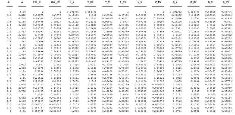
the maximum difference between flow variables for conservative and nonconservative form

Comparison of steady-state results in conservative V/S Nonconservative form at throat section
| `rho^**/ rho_o` | `T^**/ T_o` | `P^**/ P_o` | `M` | |
|
Exact analytical solution |
0.634 | 0.833 | 0.528 | 1.000 |
|
Conservation form, numerical results (31 points) |
0.65238 | 0.84107 | 0.5487 | 0.97799 |
|
Nonconservation form, numerical results (31 points) |
0.63866 | 0.83645 | 0.53421 | 0.99939 |
|
Conservation form, numerical results (61 points) |
0.63899 | 0.83566 | 0.53398 | 0.99783 |
|
Nonconservation form, numerical results (61 points) |
0.63766 | 0.83544 | 0.53273 | 0.99978 |
Graphs:-
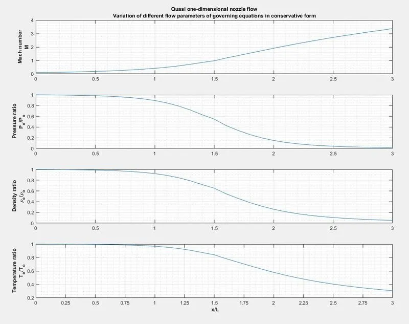
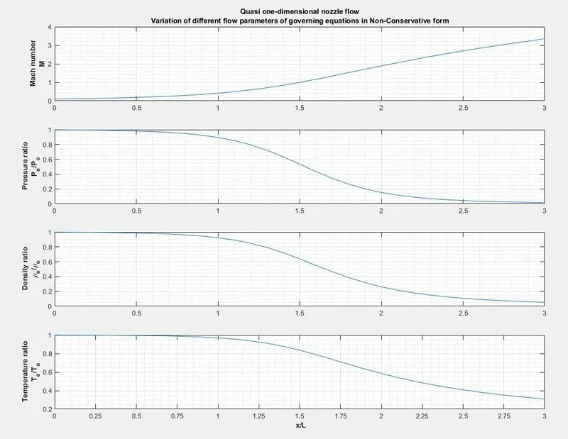
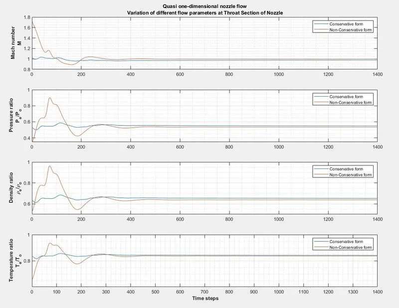
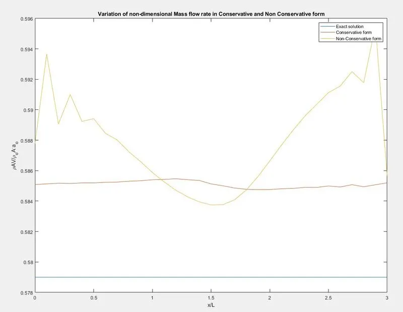
conclusions:-
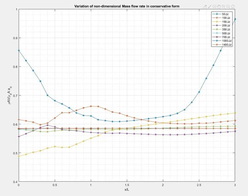
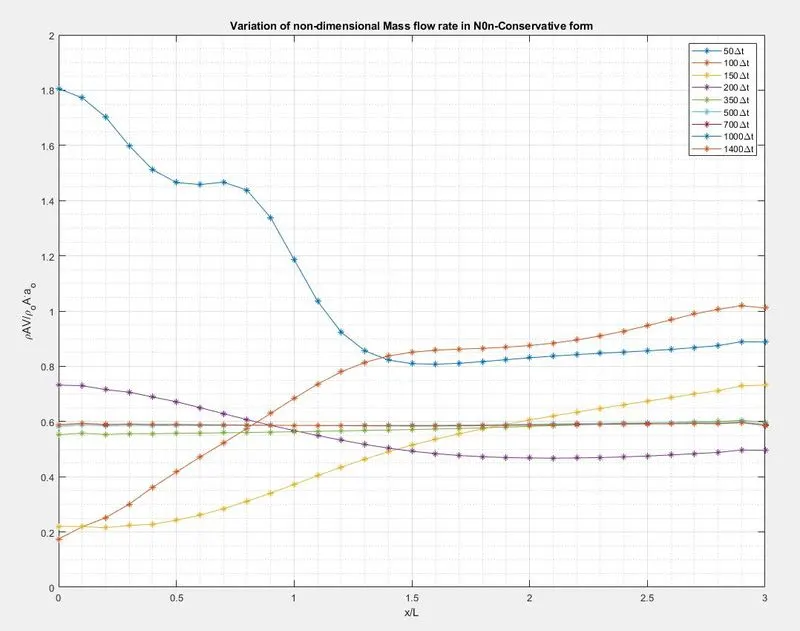
The conservation form does a better job of preserving mass throughout the flow field, mainly because the mass flow itself is one of the dependent variables in the equations-the mass flow is a primary result from these equations. In contrast, the dependent variables in the nonconservation form of the equations are the primitive variables, and the mass flow is obtained only as a secondary result. Because the conservation form of the equations does a better job of conserving mass throughout the flow field.
let us take a look at the primitive variables, in particular, temperature, pressure, and Mach number at the nozzle throat. The nonconservation form results are distinctly closer to the exact values.
A comparison results for grid points (31 in comparison to 11 points) of two forms are an indication of grid independence for the conservation form results. Note that, by doubling the number of grid points, the steady-state numerical results are slightly closer to the exact, analytical values (but still not as close as the nonconservation form results with half as many grid points). For all practical purposes, we have grid independence with 31 grid points.
In summary, for the given flow problem, we cannot establish a clear superiority of the conservation form of the governing equations over the nonconservation form. In essence, from all our previous discussions, we can only make the following observations:
1. The conservation form yields a better mass flow distribution. The conservation form simply does a better job of conserving mass.
2. The nonconservation form leads to smaller residuals. The amount by which the residuals decay is often used as an index of the "quality" of the numerical algorithm. In this sense, the nonconservation form does a better job.
3. There is no clear superiority of either form in terms of the accuracy of the results. The nonconservation form seems to produce slightly more accurate results for the primitive variables, and the conservation form seems to produce slightly more accurate results for the flux variables. The results, in either case, are certainly satisfactory
4. Comparing the amount of calculational effort to achieve a solution, we note that the solution of the conservation form requires marginally more work. Most of this is due to the need to decode the primitive variables from the flux variables, such decoding is not necessary when you are solving the nonconservation form.