Simulation of a 1D Super-sonic nozzle flow simulation using Macormack Method

Aim

• To simulate the isentropic flow through a quasi 1D subsonic-supersonic nozzle by the Macormack method using MATLAB
• To obtain the following plots:

1. Steady-state distribution of primitive variables inside the nozzle
2. Time-wise variation of the primitive variables
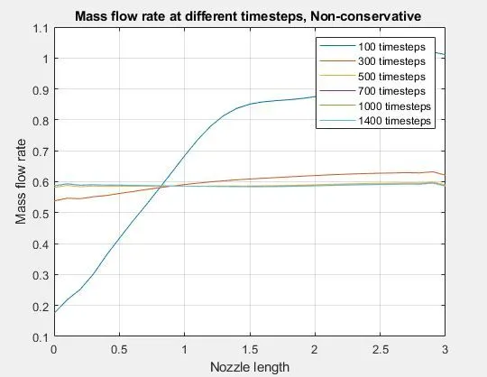
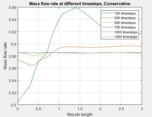
3. Variation of Mass flow rate distribution inside the nozzle at different time steps during the time-marching process
4. Comparison of Normalized mass flow rate distributions of both forms

Theory

While an analytical exact solution exists for this problem, the numerical solution is obtained to illustrate the method of CFD solving techniques.

The results are compared with those published in CFD: An introduction, by John D. Anderson.

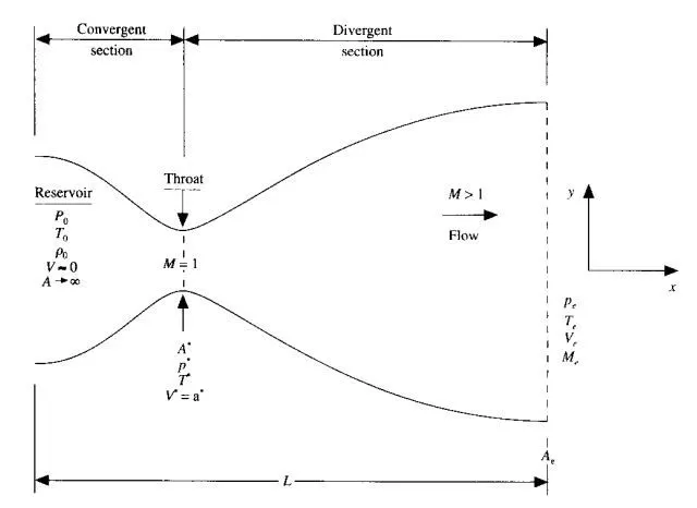
Steady isentropic flow is considered through a standard nozzle. Inlet flow comes from a resevoir with pressure and temperatures p0 and t0 respectively.

The governing equations (expressed as partial differential equations) are represented in two forms, the conservative and non conservative forms.

Non conservative:

Continuity

Momentum

Energy

Conservative:

Continuity

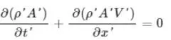
Momentum

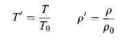
In the equations, the prime represents non dimensionalised forms of different quantities.

Energy

Non dimensional temperature and density:

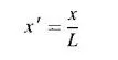
Dimensionless length:

Speed of sound:

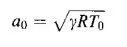
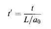
Dimensionless time:

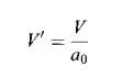
Dimesnionless velocity:

Dimensionless area:

Finite difference methods are used to solve the governing equations by the Macormack method.

The general steps to solve this problem are:

Meshing: Creating of gridpoints or a mesh, in this case 31 points.

Discretization: The pde's are solved for each element using the Macormack method. This method involves the following steps, (which can be better understood from the code):

1. Predictor step, using forward differencing
2. Corrector step, using backward differening
3. Time average derivative of the predictor and corrector step
4. Final solution update

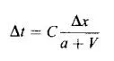
Time step size control is implemented using the Courant number (C) criteria. For this problem, C<=5 provides stable results.

Solving the PDE's by applying intial and boundary conditions:

For the non conservative form, the intial conditions are:

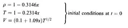
Boundary conditions:

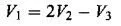(at the first grid point)

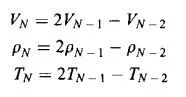(at the n'th grid point)

For the conservative form, the intial conditions are:

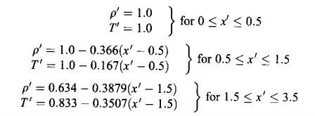
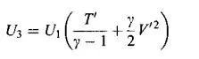
Also, the governing equations have been modified in terms of solution vector U, flux vector F, and source term J as follows:

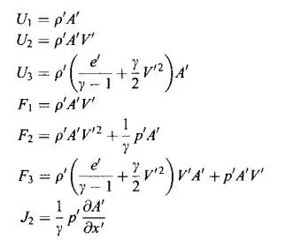
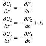
Thus the governing equations are now:

Also, it can be seen that

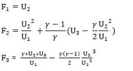
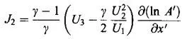
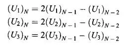
Boundary conditions:

Program

%1D Nozzle flow main code
clear all
close all
clc

%------------------------------------------------------------------>inputs
n = 31; %number of grid points
gamma = 1.4;
x = linspace(0,3,n);
dx = x(2) - x(1);
nt = 1400; %number of timesteps

%non conservative form
[rho_nc,v_nc,t_nc,mass_flow_nc,mach_nc,pressure_nc,rho_throat_nc,t_throat_nc,v_throat_nc,mass_flow_nc_throat,pressure_nc_throat, mach_nc_throat] = non_conservative_form(x,n,dx,nt,gamma);

%conservative form
[rho_c,v_c,t_c,mass_flow_c,mach_c,pressure_c,rho_throat_c,t_throat_c,v_throat_c,mass_flow_c_throat,pressure_c_throat, mach_c_throat] = conservative_form(x,n,dx,nt,gamma);




%------------------------------------------------------------------> plots

%------> Steady-state distribution of primitive variables inside the nozzle
%temperature
figure(1)
subplot(4,1,1)
grid on;
title('Steady-state distribution of primitive variables inside the nozzle')
plot(x,t_nc)
hold on
plot(x,t_c,'*')
xlabel('Nozzle length')
ylabel('Temperature')
%density
subplot(4,1,2)
grid on;
plot(x,rho_nc)
hold on
plot(x,rho_c,'*')
xlabel('Nozzle length')
ylabel('Density')
%mach number
subplot(4,1,3)
grid on;
plot(x,mach_nc)
hold on
plot(x,mach_c,'*')
xlabel('Nozzle length')
ylabel('Mach number')
%pressure 
subplot(4,1,4)
grid on;
plot(x,pressure_nc)
hold on
plot(x,pressure_c,'*')
xlabel('Nozzle length')
ylabel('Pressure')
legend('Non-conservative form','Conservative form')


%------> timewise variation of primitive variables inside the nozzle
range_timesteps = linspace(1,nt,nt);
%temperature
figure(2)
subplot(4,1,1)
grid on;
title('Timewise variation of primitive variables inside the nozzle')
plot(range_timesteps,t_throat_nc)
hold on
plot(range_timesteps,t_throat_c,'g')
xlabel('Number of timesteps')
ylabel('Temperature')
%density
subplot(4,1,2)
grid on;
plot(range_timesteps,rho_throat_nc)
hold on
plot(range_timesteps,rho_throat_c,'g')
xlabel('Number of timesteps')
ylabel('Density')
%mach number
subplot(4,1,3)
grid on;
plot(range_timesteps,mach_nc_throat)
hold on
plot(range_timesteps,mach_c_throat,'g')
xlabel('Timesteps')
ylabel('Mach number')
%pressure 
subplot(4,1,4)
grid on;
plot(range_timesteps,pressure_nc_throat)
hold on
plot(range_timesteps,pressure_c_throat,'g')
xlabel('Number of timesteps')
ylabel('Pressure')
legend('Non-conservative form','Conservative form')

%---------------------------------------> comparison of mass flow rates
figure(5)
plot(x,mass_flow_c)
hold on
plot(x,mass_flow_nc)
title('Comparison of mass flow rates along length of nozzle')
xlabel('Nozzle length')
ylabel('Mass flow rate')
legend('Conservative form','Non-Conservative form')
grid on

This is the main program that calls functions which are seperately defined for the conservative and non conservative forms of governing equations.

Inputs are provided in the start of the code which are used by the functions to obtain the desired outputs.

Plots are created as defined in the aim.

The functions created are:

Non-Conservative form

function [rho_nc,v_nc,t_nc,mass_flow_nc,mach_nc,pressure_nc,rho_throat_nc,t_throat_nc,v_throat_nc,mass_flow_nc_throat,pressure_nc_throat, mach_nc_throat] = non_conservative_form(x,n,dx,nt,gamma)

%inditial conditions 
rho_nc = 1 - 0.3146.*x;
t_nc = 1 - 0.2314.*x; %Temperature
v_nc = (0.1 + 1.09.*x).*t_nc.^0.5;
a = 1+ 2.2*(x-1.5).^2;
throat = find(a==1);

%courant number and picking the timestep
C = 0.5;
dt = min(C*(dx./((t_nc.^0.5)+v_nc)));


%outer time loop
for k = 1:nt
    
    rho_old_nc = rho_nc;
    v_old_nc = v_nc;
    t_old_nc = t_nc;
    
    %predictor loop
    for j = 2:n-1
        dvdx = (v_nc(j+1)-v_nc(j))/dx;
        drhodx = (rho_nc(j+1)-rho_nc(j))/dx ;
        
        dtdx = (t_nc(j+1)-t_nc(j))/dx ; 
        dlogadx = (log(a(j+1))-log(a(j)))/dx ; 
        
        %continuity
        drhodt_p(j) = -rho_nc(j)*dvdx - rho_nc(j)*v_nc(j)*dlogadx - v_nc(j)* drhodx;
        
        %momentum
        dvdt_p(j) = -v_nc(j)*dvdx - (1/gamma)*(dtdx + (t_nc(j)/rho_nc(j))*drhodx);
        
        %energy
        dtdt_p(j) = -v_nc(j)*dtdx - (gamma-1)*t_nc(j)*(dvdx + v_nc(j)*dlogadx);
        
        %solution update
        rho_nc(j) = rho_nc(j) + drhodt_p(j)*dt;
        v_nc(j) = v_nc(j) + dvdt_p(j)*dt;
        t_nc(j) = t_nc(j) + dtdt_p(j)*dt;
    end
    
    %corrector loop
    for j = 2:n-1
        dvdx = (v_nc(j)-v_nc(j-1))/dx ; 
        drhodx = (rho_nc(j)-rho_nc(j-1))/dx ;
        
        dtdx = (t_nc(j)-t_nc(j-1))/dx ; 
        dlogadx = (log(a(j))-log(a(j-1)))/dx ; 
        
        %continuity
        drhodt_c(j) = -rho_nc(j)*dvdx - rho_nc(j)*v_nc(j)*dlogadx - v_nc(j)* drhodx;
        
        %momentum
        dvdt_c(j) = -v_nc(j)*dvdx - (1/gamma)*(dtdx + (t_nc(j)/rho_nc(j))*drhodx);
        
        %energy
        dtdt_c(j) = -v_nc(j)*dtdx - (gamma-1)*t_nc(j)*(dvdx + v_nc(j)*dlogadx);
        
    end
   
   %average time derivative
   drhodt = 0.5*(drhodt_p+drhodt_c);
   dvdt = 0.5*(dvdt_p+dvdt_c);
   dtdt = 0.5*(dtdt_p+dtdt_c);
   
   % solution update
   for i = 2:n-1
        rho_nc(i) = rho_old_nc(i) + drhodt(i)*dt;
        v_nc(i) = v_old_nc(i) + dvdt(i)*dt;
        t_nc(i) = t_old_nc(i) + dtdt(i)*dt;
   end
   
   
   %boundary conditions
   %inlet
   v_nc(1) = 2*v_nc(2)-v_nc(3);
   
   %outlet
   rho_nc(n) = 2*rho_nc(n-1)-rho_nc(n-2);
   v_nc(n) = 2*v_nc(n-1)-v_nc(n-2);
   t_nc(n) = 2*t_nc(n-1)-t_nc(n-2);
   
   mass_flow_nc = rho_nc.*a.*v_nc;
   mach_nc = v_nc./(t_nc.^0.5);
   pressure_nc = rho_nc.*t_nc;
   
   rho_throat_nc(k) = rho_nc(throat);
   t_throat_nc(k) = t_nc(throat);
   v_throat_nc(k) = v_nc(throat);
   mass_flow_nc_throat(k) = mass_flow_nc(throat);
   pressure_nc_throat(k) = pressure_nc(throat);
   mach_nc_throat(k) = mach_nc(throat);
   
   figure(3)
   if k == 100
       plot(x, mass_flow_nc)
       hold on;
   elseif k == 300
       plot(x, mass_flow_nc)
       hold on;
   elseif k == 500
       plot(x, mass_flow_nc)
       hold on;    
   elseif k == 700
       plot(x, mass_flow_nc)
       hold on;    
   elseif k == 1000
       plot(x, mass_flow_nc)
   elseif k == 1400
       plot(x, mass_flow_nc)
   end
   
   title('Mass flow rate at different timesteps, Non-conservative ')
   xlabel('Nozzle length')
   ylabel('Mass flow rate')
   legend('100 timesteps','300 timesteps','500 timesteps','700 timesteps','1000 timesteps','1400 timesteps')
   grid on;
   


     
end
   
   

end

Conservative form

function [rho_c,v_c,t_c,mass_flow_c,mach_c,pressure_c,rho_throat_c,t_throat_c,v_throat_c,mass_flow_c_throat,pressure_c_throat, mach_c_throat] = conservative_form(x,n,dx,nt,gamma)

%intial conditions
for p = 1:n
    if (x(p) >= 0 && x(p) <= 0.5)
        rho_c(p) = 1;
        t_c(p) = 1;
    elseif (x(p) >=0.5 && x(p) <= 1.5)
        rho_c(p) = 1 - 0.366*(x(p)-0.5);
        t_c(p) = 1 - 0.167*(x(p)-0.5);
    elseif(x(p) >= 1.5 && x(p)<= 3)
        rho_c(p) = 0.634 - 0.3879*(x(p)-1.5);
        t_c(p) = 0.833 - 0.3507*(x(p)-1.5);
    end    
end
a = 1+ 2.2*(x-1.5).^2;
throat = find(a==1);
v_c = 0.59./(rho_c.*a);
pressure_c = rho_c.*t_c;
u1 = rho_c.*a;
u2 = rho_c.*a.*v_c;
u3 = rho_c.*a.*(t_c./(gamma-1))+((gamma/2).*v_c.^2);




%time loop
for k = 1:nt
    
    %courant number and picking the timestep
    C = 0.5;
    dt = min(C*(dx./((t_c.^0.5)+v_c)));
    

    u1_old = u1;
    u2_old = u2;
    u3_old = u3;
    
    f1 = u2;
    f2 = ((u2.^2)./u1) + ((gamma - 1)/gamma)*(u3 - (gamma/2)*((u2.^2)./u1));
    f3 = ((gamma.*u2.*u3)./u1)-(gamma*(gamma-1)*((u2.^3)./(2*u1.^2)));
    
    
    %predictor loop
    for j = 2:n-1
        j2(j) = (1/gamma)*rho_c(j)*t_c(j)*((a(j+1)-a(j))/dx);
        
        %continuity
        du1dt_p(j) = -((f1(j+1)-f1(j))/dx);
        %momentum
        du2dt_p(j) = -((f2(j+1)-f2(j))/dx) + j2(j);
        %energy
        du3dt_p(j) = -((f3(j+1)-f3(j))/dx);
        
        %soln update1
        u1(j) = u1(j) + du1dt_p(j)*dt;
        u2(j) = u2(j) + du2dt_p(j)*dt;
        u3(j) = u3(j) + du3dt_p(j)*dt;
        
    end
    
    f1 = u2;
    f2 = ((u2.^2)./u1) + ((gamma - 1)/gamma)*(u3 - ((gamma*0.5*(u2.^2))./(u1)));
    f3 = ((gamma.*u2.*u3)./u1)- ((gamma*0.5*(gamma-1)*(u2.^3))./(u1.^2));
    
    %corrector loop
    for j = 2:n-1
        j2(j) = (1/gamma)*rho_c(j)*t_c(j)*((a(j)-a(j-1))/dx);
        
        %continuity
        du1dt_c(j) = -((f1(j)-f1(j-1))/dx);
        %momentum
        du2dt_c(j) = -((f2(j)-f2(j-1))/dx) + j2(j);
        %energy
        du3dt_c(j) = -((f3(j)-f3(j-1))/dx);
        
    end
    
    %time average
    du1dt = 0.5*(du1dt_c+du1dt_p);
    du2dt = 0.5*(du2dt_c+du2dt_p);
    du3dt = 0.5*(du3dt_c+du3dt_p);
    
    %final update
    for i = 2:n-1
    u1(i) = u1_old(i) + du1dt(i)*dt;
    u2(i) = u2_old(i) + du2dt(i)*dt;
    u3(i) = u3_old(i) + du3dt(i)*dt;
    end
    
    %boundary conditions
    %inlet
    u1(1) = rho_c(1)*a(1);
    u2(1) = 2*u2(2)-u2(3);
    v_c(1) = u2(1)./u1(1);
    u3(1) = u1(1)*((t_c(1)/(gamma-1))+((gamma/2)*(v_c(1)).^2));
    
    %outlet
    u1(n) = 2.*u1(n-1)-u1(n-2);
    u2(n) = 2.*u2(n-1)-u2(n-2);
    u3(n) = 2.*u3(n-1)-u3(n-2);
    
    %final soln update
    rho_c = u1./a;
    v_c = u2./u1;
    t_c = (gamma-1)*((u3./u1-(gamma/2)*(v_c).^2));
    
    
    mass_flow_c = rho_c.*a.*v_c;
    mach_c = v_c./(t_c.^0.5);
    pressure_c = rho_c.*t_c;
   
    rho_throat_c(k) = rho_c(throat);
    t_throat_c(k) = t_c(throat);
    v_throat_c(k) = v_c(throat);
    mass_flow_c_throat(k) = mass_flow_c(throat);
    pressure_c_throat(k) = pressure_c(throat);
    mach_c_throat(k) = mach_c(throat);
    
   figure(4)
   if k == 100
       plot(x, mass_flow_c)
       hold on;
   elseif k == 300
       plot(x, mass_flow_c)
       hold on;
   elseif k == 500
       plot(x, mass_flow_c)
       hold on;    
   elseif k == 700
       plot(x, mass_flow_c)
       hold on;    
   elseif k == 1000
       plot(x, mass_flow_c)
   elseif k == 1400
       plot(x, mass_flow_c)
   end
   
   title('Mass flow rate at different timesteps, Conservative')
   xlabel('Nozzle length')
   ylabel('Mass flow rate')
   legend('100 timesteps','300 timesteps','500 timesteps','700 timesteps','1000 timesteps','1400 timesteps')
   grid on;
   
end

end

First the intial conditions are established for the flow.

Next an outer timeloop is used which calculated the flow properties at every time step upto 1400

The Macormack method is used to solve the governing equations

A plot is created as defined in the aim.

Outputs

• Steady-state distribution of primitive variables inside the nozzle

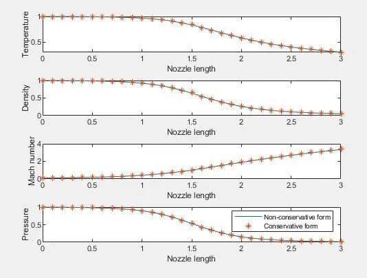
It can be observed that pressure, density and temperature have similar variations across the length of the nozzle.

Mach number is equal to 1 at the throat of the nozzle, and increases across the length of the nozzle.

• Time-wise variation of the primitive variables

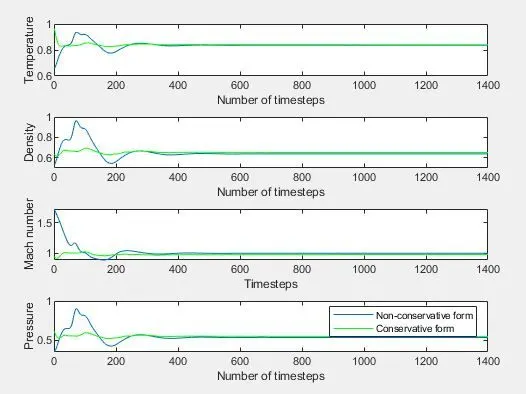
For all the primitive variables, it can be observed that it takes more timesteps to achieve a stable solution in the non-conservative case.

• Variation of Mass flow rate distribution inside the nozzle at different time steps during the time-marching process

• Comparison of Normalized mass flow rate distributions of both forms

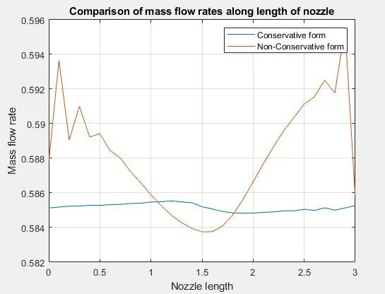
It can be observed that the solution is more stable in the conservative form along the length of the nozzle than the non-conservative form.

Grid independence test

Solution at throat after 1400 timesteps is recorded and compared with the published results.

Non-conservative form:

Number of grid points	Density	Pressure	Temperature	Mach number
n = 31	0.6387	0.5342	0.8365	0.9994
n = 61	0.6377	0.5327	0.8354	0.9998
Actual Solution	0.634	0.528	0.833	1

Conservative form:

Number of grid points	Density	Pressure	Temperature	Mach number
n = 31	0.6516	0.5478	0.8406	0.9795
n = 61	0.6383	0.5331	0.8351	0.9992
Actual Solution	0.634	0.528	0.833	1

It can be observed that changing the number of grid points provides similar results as those published in the exact solution.