Exhaust Port

Conjugate Heat Transfer in an exhaust port

Aim:

1. To understand the phenomenon of Conjugate heat transfer
2. To simulate the flow in an exhaust manifold
3. To obtain a visual representation of the process by plotting the velocity and temperature contours

Introduction:

Generally, in solid objects, heat transfer occurs by conduction whereas in fluids, convection is the governing process for heat transfer. Combining solids and fluids involves the process of Conjugate Heat Transfer (CHT), where variations of temperature occur between solids and fluids due to thermal interaction.

CHT analysis plays an essential role in analyzing this thermal interaction and is done to simulate and understand the process of CHT. It is used to study processes such as flow through a heat exchanger, a radiator, or in this simulation’s case, an exhaust manifold. All these processes involve the flow of fluid inside a solid body, and there are several thermal interactions that take place between the fluid and solid, that is, CHT. A common application involves improving the performance of cooling water jacket of an engine.

This experiment will deal with the study of CHT in an exhaust manifold.

Procedure:

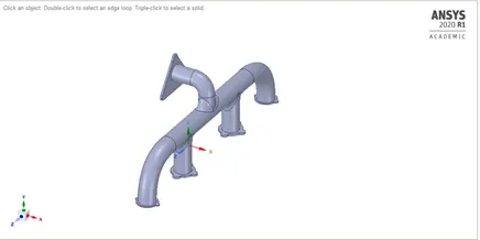
Model

Baseline Simulation

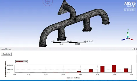
Mesh

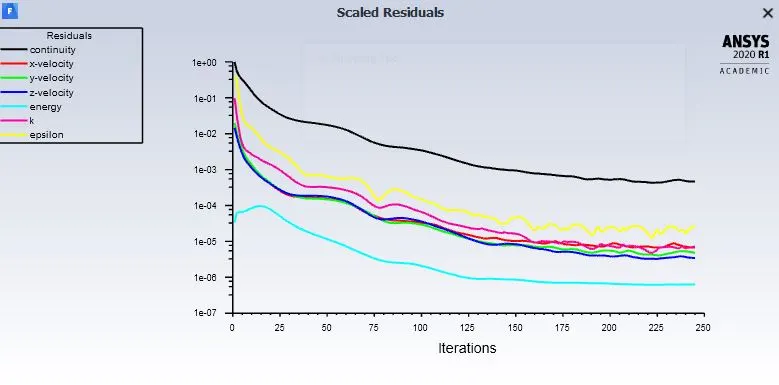
Processing

Details

Inlet conditions: Temperature = 700k

Velocity = 5 m/s

Pressure based solver

Turbulence model: K epsilon

Convection wall coefficient = 20 W/m^2 K

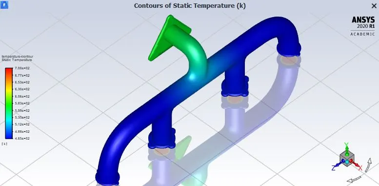
Post processing

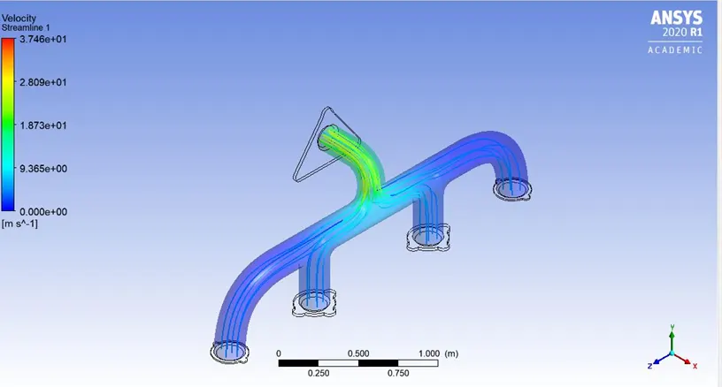
A higher velocity is observed, as explained by the continuity equation.

Let inlets be at Velocity V1, V2, V3, V4

Outlet Velocity = V

Based on continuity,

AV1 + AV2 + AV3 + AV4 = AV

Therefore, V1 + V2 + V3 + V4 = V

Due to the higher velocity at outlet, the Reynolds number at this region will be higher.

This leads to a higher heat transfer coefficient leading to a higher heat transfer from the fluid to the solid at that region.

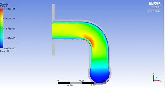
From the above figure, we can conclude that the region with the highest velocity would have the highest wall heat transfer coefficient.

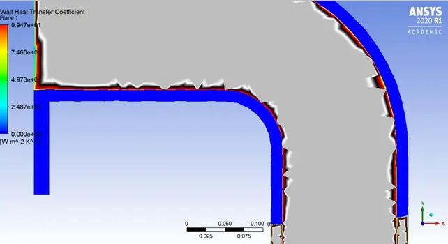
Maximum wall heat transfer coefficient is recorded as 99.46 W/m^2 K

A poor quality wall heat transfer coefficient contour is visible due to the absence of inflation layers

Refined case

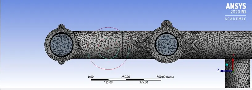
The finest possible mesh has been used.

An inflation layer, no. of layers = 6, total thickness = 5 mm has been created in order to maintain a low y+ range of between 0-5. This is ideal in order to capture values close to the wall, in the viscous sub layer.

Processing

The turbulence model has been changed, for the following reason

K omega SST is preferred in this case as it gives more accurate predictions near the wall. We require to study the wall heat transfer coefficient. As K epsilon is generally used predict values far from the wall, K omega SST is used.

Remaining conditions remain the same.

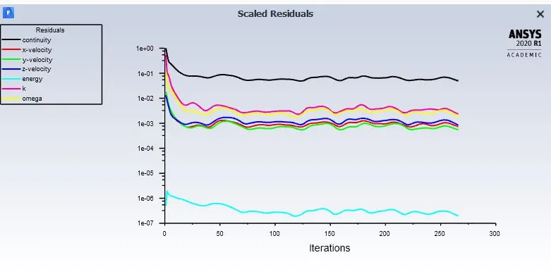
An inflation layer has been added in order to capture the contour for wall heat transfer coefficient.

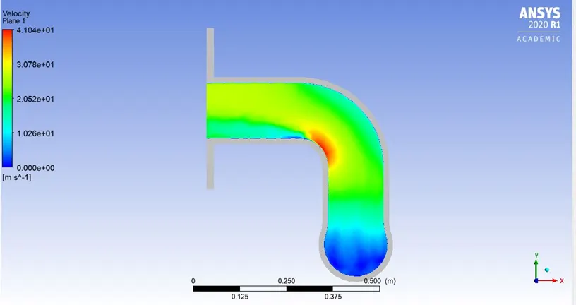
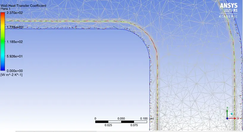
Wall heat transfer coefficient = 237 W/m^2 K

Inferences

1. Wall heat transfer coefficient is better recorded using the K omega SST model as it predicts values near the wall.
2. Velocity increases at the outlet due to conservation of energy, based on continuity equation.
3. The CHT analysis is proper because velocity and temperature increases at the output, which is expected and follows the conservation law.
4. Experimental data can also be used for comparison.