Week 7 - Simulation of a 1D Super-sonic nozzle flow simulation using Macormack Method
Simulation of 1D Subsonic-Supersonic Nozzle flow using Macormack method :
Aim : To perform a simulation on a C-D nozzle using macormack tecnique by solving the governing equations in both the non-conservative and conservative form and compare the results.
Objectives :
- Compare the results obtained for the non-conservation form and conservation form and justify the preference for the conservation form.
- Plot the steady state distribution of the property values
- Variation of the Mass flow rate distribution inside the nozzle.
Theory :
Quasi 1D flow :
A quasi 1D flow is one in which all the variables vary primarily along one direction. In our case the flow variables vary along the length direction (+ ve x-direction).
In our case of converging-diverging(C-D) nozzle, the area (A) is a function of x which varies for the given length of the nozzle as follows :
`A = 1 + 2.2*(x - 1.5)^2`
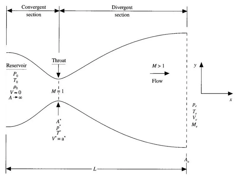
Fig.1 : Crosssection of a C-D nozzle [extracted from "CFD : The basics with applications, John.D.Anderson,Jr.]
The nozzle has a convergent section, throat and a diverging section. In the convergent section the Mach number is less than 1(M<1). Hence the flow in convergent section is subsonic.
At the throat, the Mach number is equal to 1 (M = 1). This means the flow is sonic.
Exactly after the throat, the flow becomes supersonic (M>1).
Mach number(M) :
Mach number is a dimensionless quantity which is equal to the ratio of the flow velocity to the local speed of the sound.
Mathematically, `M = u/c`
Here, u is the flow velocity and c is the velocity of the sound corresponding to the local conditions.
Assuming air as an ideal gas, the Mach number for a subsonic flow is given by :
`M = sqrt((2)/(gamma -1)*[((q_c)/(q_p)+1)^((gamma-1)/gamma) - 1])`
Here, `q_c` is the impact pressure (dynamic pressure) and
p is the static pressure
`gamma`is the ratio of specific heats at constant pressure and constant temperature respectively.
The speed of the sound varies with the temperature as `c = sqrt(gamma*R_(air)*T)`
Here, R_air is the specific gas constant for air.
For a supersonic flow, the Mach number is given by the equation:
`(p_t)/(p) = [(gamma + 1)/(2) * M^2]^((gamma)/(gamma -1) )*[(gamma + 1)/(1 - gamma + 2*gamma*M^2)]`
MacCormack technique :
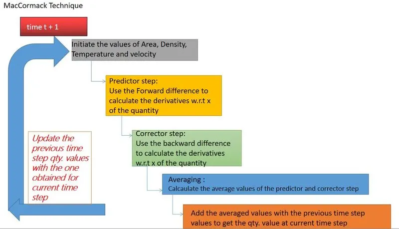
The MacCormack method predicts an intermediate value of the differential term and then using the values in the predictor step, the corrector step values are computed. After that the average value of the differential term is obtained by averaging the predictor and corrector step values. Finally the averaged value are added to the values from the previous time step so as to get the value at the next time step.
Illustration of the MacCormack technique :
Consider a sample partial differential equation :
`(delQ)/(delt) + (delQ)/(delx) = 0` - ---- ----------------------(I)
Predictor step :
Here, Q is a flow variable and the first term in the above equation represents the time rate of change of the quantity Q. The second term is the change in the quantity Q with respect to the position.
Equation I can be written as follows :
`(delQ)/(delt) = -(del Q)/(delx)`
In the predictoe step, the spatial terms are discretized as per the forward difference method
`((delQ)/(delt))_p = -(Q_(i+1) - Q_i)/(Deltax)`
In the RHS, the values of the flow quantity Q at the grid points (i+1) and (i) are from the previous time step.
Corrector step :
In the corrector step the differentials of the quantity Q are discretized as per the backward difference
`((delQ)/(delt))_c = -(Q_(i) - Q_(i-1))/(Deltax)`
Averaging :
The average values of the partial derivatives with respect to time are calculated by averaging the predictor and corrector step values.
`((delQ)/(delt))_(av) = (((delQ)/(delt))_p + ((delQ)/(delt))_c)/(2)`
Finally, the value of the Quantity at the next time step are calculated as follows
`Q^(n+1) = Q^(n) + ((delQ)/(delt))_(av) * dt`
To calculate the quantity Q at the next time step the value `Q^(n+1)` is utilized. The iterative process is repeate untill the convergence criteria is met.
Calculation of the time step dt for a courant number CFL= 0.5 :
`Deltat = C*(Deltax)/(a + V)`
Here, a is the spead of the sound
V is the local flow velocity at a point in the flow domain
`Deltax`is the grid spacing.
The `Deltat`for the velocities at each and every grid point is calculated and the minimum value of the calculated values is chosen as the actual `Delta t`
`Deltat =`minimum(`Deltat_1^t, Deltat_2^t, Deltat_3^t,.......Deltat_n^t`)
Initial and Boundary conditions:
Initial conditions:
The shape of the nozzle is held fixed and it is independent of time. Hence A = A(x) is constant throughout the simulation.
`A = 1 + 2.2*(x - 1.5)^2` `0leqxleq3`
For Density, Temperature and velocity :
`rho = 1 - 0.3146*x`
`T = 1 -0.2314*x`
`V = (0.1 + 1.09*x)*T^(0.5)`
Boundary conditions:
Inflow Boundary condition :
`V_1 = 2*V_2 - V_3`
Outflow boundary condition :
`V_N = 2*V_(N-1) - V_(N-2)`
`P_N = 2*P_(N-1) - P_(N-2)`
`T_N = 2*T_(N-1) - T_(N-2)`
Code :
% A program to simulate the quasi 1D supersonic flow in a C-D nozzle
clear; close all;clc

% Defining the grid conditions
n = 31;
x = linspace(0,3,n);
gamma = 1.4;
th = (n-1)/2;
t_list = 1:1400;

% Calling the function files conservative and non-conservative which
% compute the values of primitive variables v, t, rho, mass flow rate(m) and Mach number
[rho_c,v_c,t_c, m_c,M_c,p_c,t_th_c, rho_th_c, p_th_c, M_th_c] = conservative(n,x,gamma);
[rho_nc, v_nc, t_nc,m_nc,M_nc,p_nc,t_th_nc,rho_th_nc,p_th_nc,M_th_nc] = nonconservative(n,x,gamma);

figure(3)
subplot(4,1,1)
hold on
plot(x,rho_nc);
xlabel('Non dimensional distance');
ylabel('Density ratio');
grid minor;

subplot(4,1,2)
hold on
plot(x,t_nc);
xlabel('Non dimensional distance');
ylabel('Temperature ratio');
grid minor;

subplot(4,1,3)
plot(x,p_nc);
xlabel('Non dimensiona; distance');
ylabel('pressure ratio');
grid minor;

subplot(4,1,4)
plot(x,M_nc);
xlabel('Non dimensional distance');
ylabel('Mach number');
grid minor
sgtitle('Steady state distribution of the primitive variables in nozzle:non-conservative form');

figure(4)
subplot(4,1,1)
hold on
plot(x,rho_c);
xlabel('Non dimensional distance');
ylabel('Density ratio');
grid minor;

subplot(4,1,2)
hold on
plot(x,t_c);
xlabel('Non dimensional distance');
ylabel('Temperature ratio');
grid minor;

subplot(4,1,3)
plot(x,p_c);
xlabel('Non dimensiona; distance');
ylabel('pressure ratio');
grid minor;

subplot(4,1,4)
plot(x,M_c);
xlabel('Non dimensional distance');
ylabel('Mach number');
grid minor
sgtitle('Steady state distribution of the primitive variables in nozzle: conservative form');

figure(5)
hold on
plot(x,m_c);
plot(x,m_nc);
title('Comparison of non-dimensional mass flow rates in nozzle');
legend('conservative form','non conservative form');

figure(6)
subplot(4,1,1)
grid on
plot(t_list,t_th_c);
ylabel('y/y_0');
legend('Temperature');
title('Timwise variation of the temperature at throat');
grid minor

subplot(4,1,2)
grid
plot(t_list,p_th_c);
ylabel('p/p_0');
title('timewise variation of the pressure at the throat');
legend('Pressure');
grid minor

subplot(4,1,3)
grid
plot(t_list,rho_th_c);
ylabel('rho/rho_0');
title('timewise variation of the density at the throat');
legend('density');
grid minor

subplot(4,1,4)
grid
plot(t_list,M_th_c);
ylabel('Mach Number');
title('timewise variation of the Mach number at the throat');
legend('Mach number');
grid minor

sgtitle('Timewise varaition of the primitive variables - Conservative form')


figure(7)
subplot(4,1,1)
grid on
plot(t_list,t_th_nc,'color','r');
ylabel('y/y_0');
legend('Temperature');
title('Timwise variation of the temperature at throat');
grid minor

subplot(4,1,2)
grid
plot(t_list,p_th_nc,'color','r');
ylabel('p/p_0');
title('timewise variation of the pressure at the throat');
legend('Pressure');
grid minor

subplot(4,1,3)
grid
plot(t_list,rho_th_nc,'color','r');
ylabel('rho/rho_0');
title('timewise variation of the density at the throat');
legend('density');
grid minor

subplot(4,1,4)
grid
plot(t_list,M_th_nc,'color','r');
ylabel('Mach Number');
title('timewise variation of the Mach number at the throat');
legend('Mach number');
grid minor

sgtitle('Timewise varaition of the primitive variables: Non-conservative form')
"Conservative.m" function file which computes the local primitive variables velocity(v), mass flow rate(m), density(`rho`), temperature(t) and the Mach number (M) using the governing equations in the conservative form.
function [rho,v,t, m, M,p,t_th, rho_th, p_th, M_th] = conservative(n,x,gamma)

dx = x(2) - x(1);
nt = 1400;
cfl = 0.5;
% Calculation of the initial values of the Density, Area and
% Temperature

%initialization of the variables for density and temperature
rho = zeros(1,n);
t = zeros(1,n);
a = 1 + 2.2*(x - 1.5).^(2);

th = find(a ==1);
% Filling the values

for ii = 1:1:6
    rho(ii) = 1;
    t(ii) = 1;
end

for ij = 7: 1: 16
    rho(ij) = 1 - (0.366*(x(ij) - 0.5));
    t(ij) = 1 - (0.167*(x(ij) - 0.5));
end

for ik = 17 : 1: 31
    rho(ik) = 0.634 - (0.3879*(x(ik) - 1.5));
    t(ik) = 0.833 - (0.3507*(x(ik) - 1.5));
end

v = 0.59./(rho.*a);

%Calculation of the solution terms
u1(1:n) = rho.*a;
u2(1:n) = 0.590;
u3(1:n) = rho.*(2.5*t + 0.7*v.^2).*a;

% Assigning the values of the solution terms to variables with 'prev'
% suffix
u1_prev = u1;
u2_prev = u2;
u3_prev = u3;

for k = 1:nt
  till = sqrt(t);
  dt_sample = (cfl*dx)./(till + v);
  dt = min(dt_sample);
     %calculation of the flux vectors
    f1(1:n) = u2;
    var1 =(u2.^2)./(u1);
    var2 = (u2.^3)./(u1.^2);
    f2 = ((u2.^2)./u1) + ((gamma - 1)/gamma)*(u3 - (gamma/2)*var1);
    f3 = ((gamma.*u2.*u3))./(u1) - ((gamma*(gamma - 1)/2)*var2);

for i = 2 : n - 1
    %source term
    j2(i) = (1/gamma).*rho(i).*t(i).*((a(i + 1) - a(i))./dx);

    du1_dt_p(i) = -(f1(i + 1) - f1(i))/dx;
    du2_dt_p(i) = -((f2(i + 1) - f2(i))/dx) + j2(i);
    du3_dt_p(i) = -(f3(i + 1) - f3(i))/dx;

    %updatation of the solution terms
    u1(i) = u1(i) + du1_dt_p(i).*dt;
    u2(i) = u2(i) + du2_dt_p(i).*dt;
    u3(i) = u3(i) + du3_dt_p(i).*dt;
end

% Decoding the primitive variables
rho = u1./a;
v = u2./u1;
t = (gamma - 1)*((u3)./(u1) - (gamma/2)*((u2./(u1)).^2));

% Corrector step
% Calculation of the fluxes f1, f2 and f3 for the corrector step
f1(1:n) = u2;
var1 =(u2.^2)./(u1);
var2 = (u2.^3)./(u1.^2);
f2 = ((u2.^2)./u1) + ((gamma - 1)/gamma)*(u3 - (gamma/2)*var1);
f3 = ((gamma.*u2.*u3))./(u1) - ((gamma*(gamma - 1)/2)*var2);


for j = 2 : n-1
    j2(j) = (1/gamma).*rho(j).*t(j).*((a(j) - a(j - 1))./dx);
    du1_dt_c(j) = -(f1(j) - f1(j - 1))/dx;
    du2_dt_c(j) = -((f2(j) - f2(j - 1))/dx) + j2(j);
    du3_dt_c(j) = -(f3(j) - f3(j - 1))/dx;
end

% Computing the average values of the time derivative of the solution terms
du1_dt = 0.5*(du1_dt_p + du1_dt_c);
du2_dt = 0.5*(du2_dt_p + du2_dt_c);
du3_dt = 0.5*(du3_dt_p + du3_dt_c);

% Calculation of the final values of the solution vectors
for l = 2 : n-1
    u1(l) = u1_prev(l) + (du1_dt(l) * dt);
    u2(l) = u2_prev(l) + (du2_dt(l) * dt);
    u3(l) = u3_prev(l) + (du3_dt(l) * dt);
end


% Extraction of the temperatue, velocity and density from the final
% solution terms
rho = u1./a;
v = u2./u1;
t = (gamma - 1)*((u3)./(u1) - (gamma/2)*((u2./(u1)).^2));
m = rho.*a.*v;
M = v./sqrt(t);
p = rho.*t;
% Implementing the boundary conditions

% Inlet boundary conditions
u1(1) = a(1);
u2(1) = 2*u2(2) - u2(3);
v(1) = u2(1)/u1(1);
u3(1) = u1(1)*((t(1))/(gamma - 1) + (gamma/2)*v(1)^2);

%outlet boundary conditions
u1(n) = 2*(u1(n-1)) -u1(n-2);
u2(n) = 2*(u2(n-1)) -u2(n-2);
u3(n) = 2*(u3(n-1)) -u3(n-2);
% Predictor step

% Assigning the values of newly extracted values of the solution terms to
% the previous time step solution terms
u1_prev = u1;
u2_prev = u2;
u3_prev = u3;

% Initialising index updatation of primitive variables at throat wrt
% increment in time steps
rho_th(k) = rho(th);
t_th(k) = t(th);
p_th(k) = p(th);
M_th(k) = M(th);

% Graph for variation of mass flow rate distribution inside the nozzle at different time steps
figure(1)
hold on
grid minor
if k == 1
  plot(x,m,'color','b')
  A1 = "initial value";
else if k == 100
  plot(x,m,'color','r')
  A2 = "100th time step";
else if k == 500
  plot(x,m,'color','g');
  A3 = "500th time step";
else if k == 1000
  plot(x,m);
  A4 = "1000th time step";
else if k == 1200
  plot(x,m)
  A5 = "1200th time step";
else if k == 1400
  plot(x,m)
  A6 = "1400th time step";
  xlabel('Non dimensional distance through nozzle');
  ylabel('Mass flow rate');
  title('Distribution of Mass flow rate inside the nozzle at various time steps');
  legend([A1,A2,A3,A4,A5,A6]);
  axis([0 3 0 1.2]);
end
end
end
end
end
end

end

end
Results :
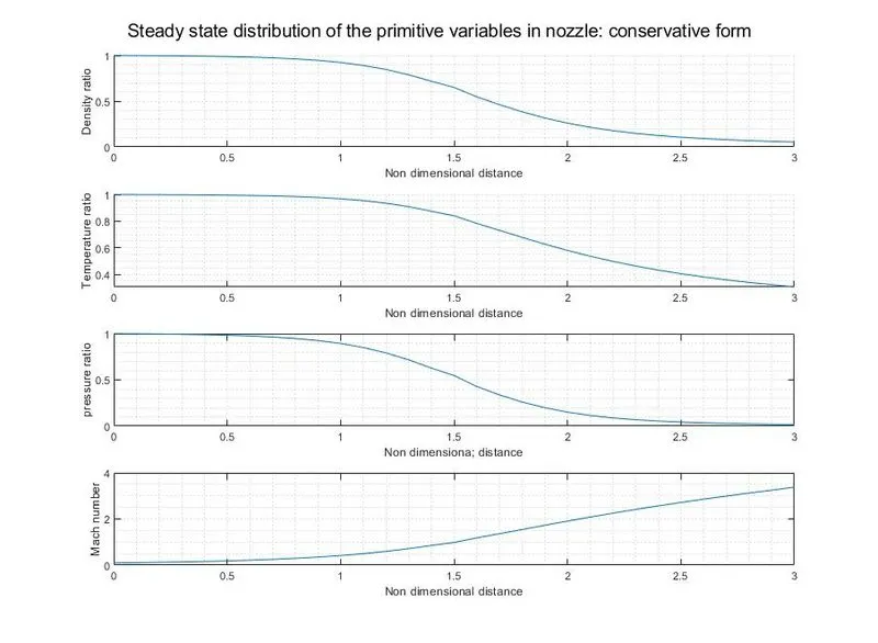
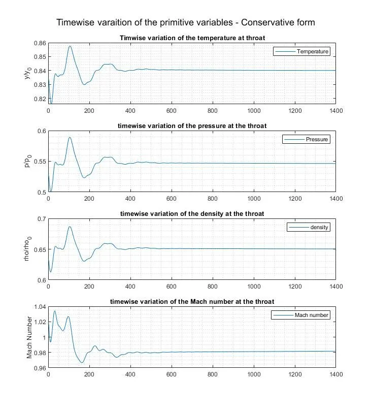
1. Plots for the local values of the primitive quantities at the steady state conditions in the conservative form
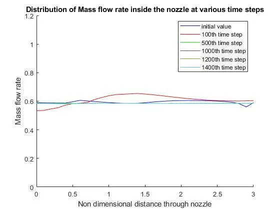
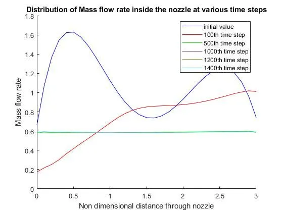
2. Variation of the Mass flow rate distribution inside the nozzle at different time steps during the time marching process.
3. Timewise variation of the flow variables at the throat of the nozzle for the conservation form
nonconservative.m function file which computes the local primitive variables velocity(v), mass flow rate(m), density(`rho`), temperature(t) and the Mach number (M) using the governing equations in the non-conservative form.
function [rho, v, t,m, M,p,t_th,rho_th,p_th,M_th] = nonconservative(n,x,gamma)


t = 1 - (0.2314*x);
v = (0.1 + 1.09*x).*(t.^(0.5));
rho = 1 - (0.3146*x);
a = 1 + 2.2*(x - 1.5).^(2);
cfl = 0.5;
th = find(a == 1);
%Determination of the time step value dt
for s = 2: length(x)
    dx(s-1) = x(s) - x(s - 1);
    dt_sample(s-1) = cfl*((dx(s - 1))/(sqrt(t(s)) + v(s)));
end
dt = min(dt_sample);
dx = min(dx);
% Time loop

nt = 1400;

% looping through the time

for k = 1 :nt
  rho_old = rho;
  t_old = t;
  v_old = v;

    % Predictor method
    for j = 2 : n - 1

    dv_dx = ((v(j + 1) - v(j))/dx);
    drho_dx = ((rho(j + 1) - rho(j))/dx);
    dt_dx = (t(j+1) - t(j))/(dx);
    d_lna_dx = ((log(a(j + 1)) -log(a(j)))/dx);

    % Continuity equation (solving for drho_dt)
    drho_dt_p(j) = -rho(j)*dv_dx - rho(j)*v(j)*d_lna_dx - v(j)*drho_dx;

    % Momentum equation
    dv_dt_p(j) = -v(j)*dv_dx - (1/gamma)*(dt_dx + (t(j)/rho(j)) * drho_dx);

    % Energy equation
    dt_dt_p(j) = -v(j)*dt_dx - (gamma - 1)*t(j)*(dv_dx + v(j)*d_lna_dx);

     % solution update

    rho(j) = rho(j) + drho_dt_p(j) * dt;
    v(j) = v(j) + dv_dt_p(j) * dt;
    t(j) = t(j) + dt_dt_p(j) * dt;
    end

 % Corrector method
    for j = 2 : n - 1

    dv_dx = ((v(j) - v(j - 1))/dx);
    drho_dx = ((rho(j) - rho(j - 1))/dx);
    dt_dx = (t(j) - t(j - 1))/(dx);
    d_lna_dx = ((log(a(j)) -log(a(j - 1)))/dx);

    % Continuity equation (solving for drho_dt)
    drho_dt_c(j) = -rho(j)*dv_dx - rho(j)*v(j)*d_lna_dx - v(j)*drho_dx;

    % Momentum equation
    dv_dt_c(j) = -v(j)*dv_dx - (1/gamma)*(dt_dx + (t(j)/rho(j)) * drho_dx);

    % Energy equation
    dt_dt_c(j) = -v(j)*dt_dx - (gamma - 1)*t(j)*(dv_dx + v(j)*d_lna_dx);

    end

  %Computation of the average value

  drho_dt = 0.5*(drho_dt_p + drho_dt_c);
  dv_dt = 0.5*(dv_dt_p + dv_dt_c);
  dt_dt  = 0.5*(dt_dt_p + dt_dt_c);

  % Final solution
  for l = 2: n-1
  rho(l) = rho_old(l) + drho_dt(l) * dt;
  v(l) = v_old(l) + dv_dt(l) * dt;
  t(l) = t_old(l) + dt_dt(l) * dt;
  end

  % Applying the boundary conditions

  % Inlet boundary condition
  v(1) = 2*v(2) - v(3);

 %Outlet boundary condition
 rho(n) = 2*rho(n-1) - rho(n-2);
 v(n) = 2*v(n-1) - v(n-2);
 t(n) = 2*t(n-1) - t(n-2);
 v_plot_l(k) = v(15);
 v_plot(k) = v(16);
 v_plot_u(k) = v(17);

 p = rho.*t;
 m = rho.*a.*v;
 M = v./sqrt(t);

 % Initialising the index updatation of primitive variables at throat wrt
 % increment in time step
 rho_th(k) = rho(th);
 t_th(k) = t(th);
 p_th(k) = p(th);
 M_th(k) = M(th);
 % Graph for variation of mass flow rate distribution inside the nozzle at different time steps
figure(2)
hold on
grid minor
if k == 1
  plot(x,m,'color','b')
  A1 = "initial value";
else if k == 100
  plot(x,m,'color','r')
  A2 = "100th time step";
else if k == 500
  plot(x,m,'color','g');
  A3 = "500th time step";
else if k == 1000
  plot(x,m);
  A4 = "1000th time step";
else if k == 1200
  plot(x,m)
  A5 = "1200th time step";
else if k == 1400
  plot(x,m)
  A6 = "1400th time step";
  xlabel('Non dimensional distance through nozzle');
  ylabel('Mass flow rate');
  title('Distribution of Mass flow rate inside the nozzle at various time steps');
  legend([A1,A2,A3,A4,A5,A6]);
  axis([0 3 0 2]);

end
end
end
end
end
end

end
end
Results :
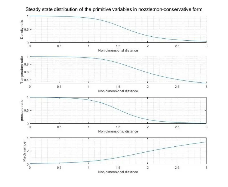
1. Plot for the local values of the primitive variables at steady state conditions - Non conservative form
2. Variation of the mass flow rate inside the nozzle at various time steps during the time marching process - Non conservation form.
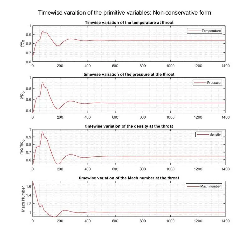
3. Timewise variation of the flow variables at the throat in the conservative form
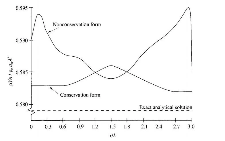
3. Comparison of Normalized mass flow rate distributions of both forms
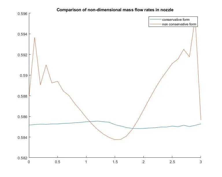
The following image is extracted from the textbook " Computational Fluid Dynamics - Basics with applications by John.D.Anderson,Jr. 2e" to compare the obtained plot for normalized mass flow rate for both the forms
Analysis :
The conservation form gives a result which is much close to the exact result and has not got the oscillations at the inlet and outlet.
Grid dependence study :
| Density ratio(`rho/rho_0`) | Temperature ratio (`T/T_0`) | Pressure ratio (`P/P_0`) | Mach number (M) | |
| Exact solution | 0.634 | 0.833 | 0.528 | 1 |
| Non-Conservation form (31 grid points) | 0.638 | 0.836 | 0.534 | 0.999 |
| Conservation form (31 grid points) | 0.652 | 0.841 | 0.548 | 0.977 |
| Non-Conservation form(61 grid points) | 0.637 | 0.835 | 0.532 | 0.999 |
| Conservation form(61 grid points) | 0.638 | 0.835 | 0.533 | 0.997 |
Conclusion:
Even though the grid points are doubled, the change in the magnitude of the flow variables is marginal. It can be roughly said that the case with 31 grid points is independent of the mesh size.
However, if greater accuracy is desired going with a fine grid would resolve the flow quantities better.
In our case, upon the increasing the grid points by two or three folds the increase in accuracy is barely noticable.