Simulation of a 1D Super-sonic nozzle flow simulation using Macormack Method
AIM:
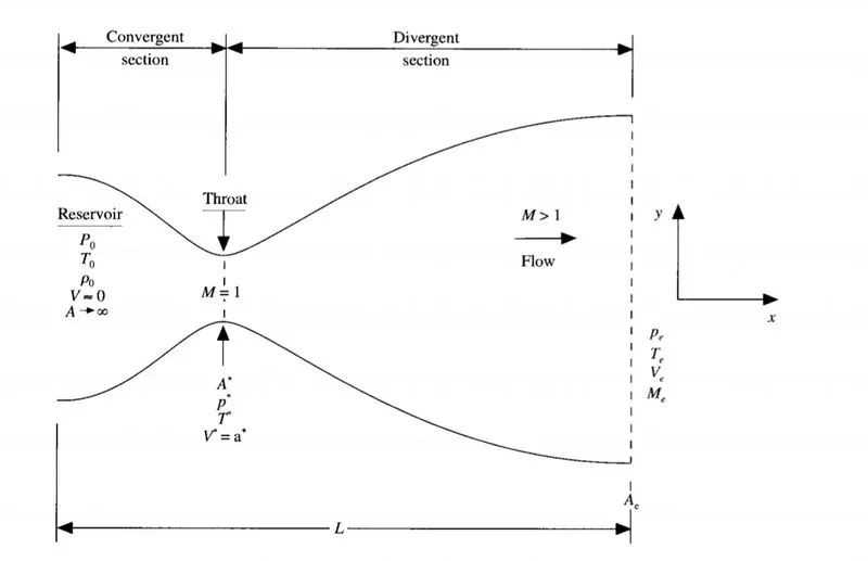
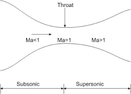
To simulate the isentropic flow through a quasi 1D subsonic-supersonic nozzle. You will derive both the conservation and non-conservation forms of the governing equations and solve them using the MacCormack's technique.
OBJECTIVE:
You need to determine the steady-state temperature distribution for the flow-field variables and investigate the difference between the two forms of governing equations by comparing their solutions.
You need to show the following plots inside your report
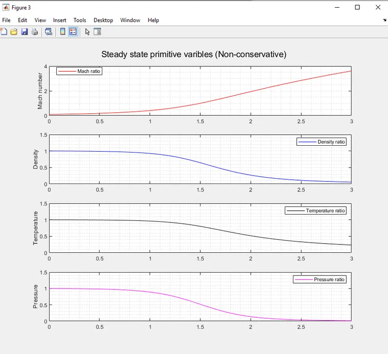
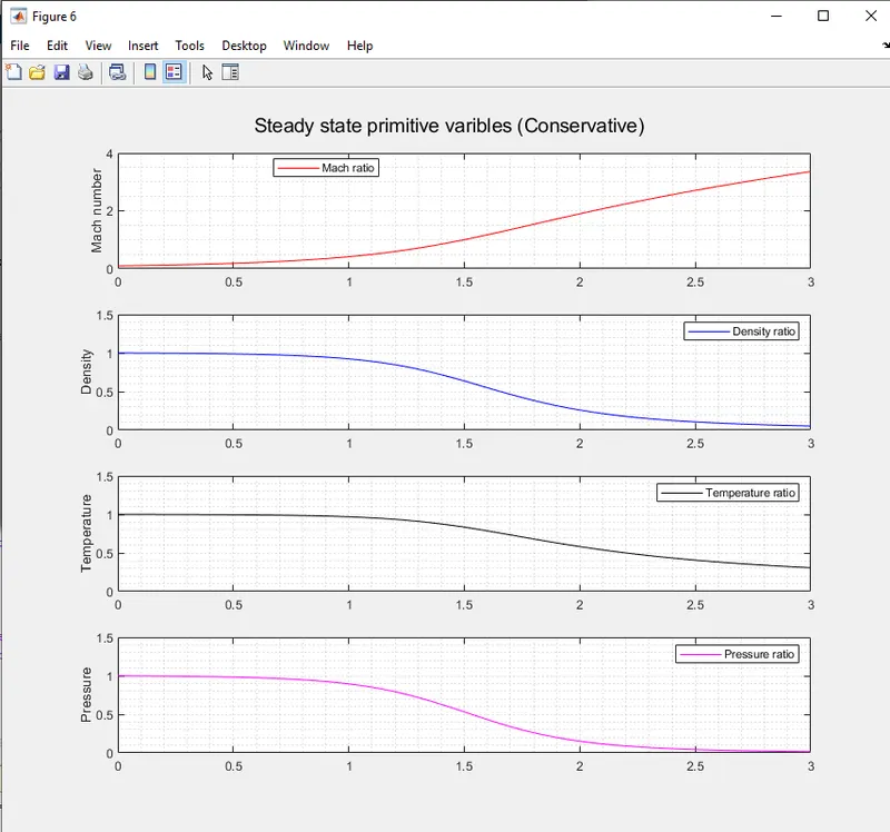
1. Steady-state distribution of primitive variables inside the nozzle
2. Time-wise variation of the primitive variables
3. Variation of Mass flow rate distribution inside the nozzle at different time steps during the time-marching process
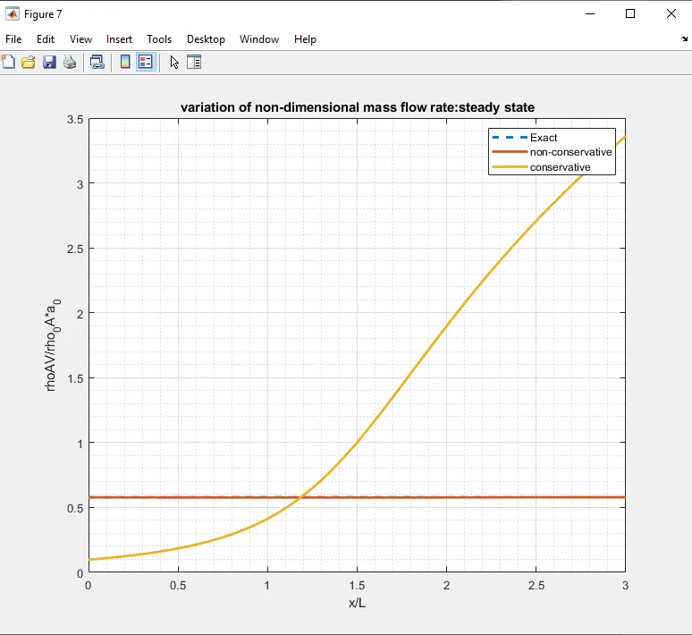
4. Comparison of Normalized mass flow rate distributions of both forms
EQUATIONS:
- Non- Conservative form:
- Continuity equation:
`(∂ρ)/(∂t)= -ρ'(∂v)/(∂x)-ρ'v'(∂(lnA'))/(∂x)-v'(∂p)/(∂x)`
2. Momentum equation:
`(∂v)/(∂t)= -v'(∂v)/(∂x)-1/γ(∂T)/(∂x)+(T')/(ρ') (∂ρ)/(∂x)`
3. Energy equation:
`(∂T')/(∂t)= -v'(∂T')/(∂x)-(γ-1)T'(∂v')/(∂x)+v'(∂(lnA'))/(∂x)`
2. Conservation form:
1. Continuity equation:
`(∂(ρ'A'))/(∂t)+(∂(ρ'A'v'))/(∂x)`
2. Momentum equation:
`(∂(ρ'A'v'))/(∂t)+(∂(ρ'A'v'^2+(1/γ)p'A'))/(∂x)=1/γ p'(∂A')/(∂x)`
3. Energy equation:
`(∂(ρ'A'(e^'/(γ-1)+γ/2 v'^2 )))/(∂t)+(∂(ρ'(e^'/(γ-1)+γ/2 v'^2 )v'A'+p'A'v'))/(∂x)=0`
The above conservative equations can be made easier to compute by assigning larger terms to certain variables. Therefore, certain terms can be easily converted into the following terms.
a. Solution variables,
U1= ρ’A’
U2= ρ’A’v’
`U3= ρ'A'((e')/(γ-1)+γ/2 v'^2)`
b.Flux variables,
F1= ρ’A’v’
`F2= ρ'A'v'^2+ 1/γ p'A'`
`F3= ρ'A'v'(e^'/(γ-1)+(γv^'2)/2)+ρ'A'v'`
`J2= 1/γ p'(∂A)/(∂x)`
Now with these equations, we can re-write the conservative form as,
`(∂U1)/(∂t)= -(∂F1)/(∂x)`
`(∂U2)/(∂t)= -(∂F2)/(∂x)+J2`
`(∂U3)/(∂t)= -(∂F3)/(∂x)`
3. Non- dimensional quantities:
Also as part of our problem setup we represent quantities in terms of non-dimensional quantities. This way it makes us easier to solve the problem w.r.t to coding and also with no depending variables.
a. Temperature, `T'=T/T_0`
b. Density, `ρ^'= ρ/ρ_0`
c. Non-dimensional distance, `x^'= x/L`
d. Non-dimensional velocity, `v^'= v/a_0` Where ‘`a_0`' is the local speed of sound(`a_0= √γRT_0`)
e. Non-dimensional time, `t^'= t/(L/a_0 )`Where ‘`L/a_0`’ is the characteristic time scale
f. Non-dimensional area, `A^'= A/A^*`
THEORY:
1. MacCormack method:
In computational fluid dynamics, the MacCormack method is a widely used discretization scheme for the numerical solution of hyperbolic PDE's. This second-order finite difference method was introduced by Robert W. MacCormack in 1969. The MacCormack method is elegant and easy to understand and program.
MacCormack's technique is a variant of the Lax-Wendroff approach but is much simpler in its application. The Maccormack method is also an explicit finite-difference technique which is second-order-accurate in both space and time. First introduced in 1969, it became the most popular explicit finite-difference method for solving fluid flows for the next 15 years. Today, the Maccormack method has been mostly supplanted by more sophisticated approaches. However, the Maccormack method is very "student-friendly" it is among the easiest to understand and program. Moreover, the results obtained by using MacCormack'smethod are perfectly satisfactory for many fluid flow applications. For these reasons, MacCormack's method is highlighted here and will be used for some.
The MacCormack method consists of 3 stages,
a. Initial conditions.
b. Predictor Step.
c. Corrector step.
a. Initial conditions: the initial conditions are given with respect to non-dimensional form which is,
rho= 1-0.3146x
T= 1-0.2314x
`V= (0.1 + 1.09x)T^(1/2)`
`A= 1 + 2.2(x-1.5)^2` where, 0<=x<=3
pressure, p= p'T'
Mach Number, M=`(v')/ sqrt T'`
after initialising the initial conditions, we are asked to calculate the predictor and corrector step
b. Predictor step:
In the predictor step, a "provisional" value of u at time level n+1 (denoted by  ) is estimated as follows

The above equation is obtained by replacing the spatial and temporal derivatives in the previous first-order hyperbolic equation using forward differences.
c. Corrector step: In the corrector step, the predicted value is corrected according to the equation

Note that the corrector step uses backward finite difference approximations for spatial derivative. The time-step used in the corrector step is  in contrast to the
  used in the predictor step.
Replacing the  term by the temporal average

to obtain the corrector step as

After the corrector step is calculated the average value is calculated of both the predictor and the corrector step, and after calculating the average the final value for that time step can be calculated as follows,
`Function(f)^(2nd-time-step) = f(1st) + (delF)/(delt)avg . deltat`
- The Solution of the problem has 3 phases
1. Mesh
2. Discretise
3. Solution ( initial conditions and boundary conditions)
Initially, a 1D mesh is created with necessary nodes and boundary conditions(inlet- subsonic inlet, outlet- supersonic outlet)
- Code Explanation:
1. Initially, 2 separate functions are created for a conservative and non-conservative form of equations
2. The necessary values are obtained and the graphs are plotted under conservative and non-conservative forms.
3. A main program is created the functions are called and call the necessary graphs to be viewed.
4. After the necessary values are called from the functions, the graph can be plotted for conservative v/s non-conservative.
- CODE:
1. Main program:
% Main program for simulation of 1D super-sonic nozzle

clear all
close all
clc


%Area at throat
n=61;
x=linspace(0,3,n);
n_throat= (n-1)/2;
nt= 1400;   %time steps


%Non-Conservative
tic
[mass_flow, rho, Temp, p, M]= non_conser_nozzle(n,nt,n_throat);
t1= toc;

fprintf('Computation time (non- conservative)= %0.3f sec', t1);

%Conservative
tic
[rho2,T2,P2,M2,m2]=Quasi_1D_nozzle_flow_conservative_func(n,nt,n_throat);
t2=toc;

fprintf('nn')
fprintf('Computation time (Conservative)= %0.3f sec', t2);

%plotting

figure(7)

figure(7)
plot(x,0.579*ones(length(x),1),'--','Linewidth',2)
hold on
grid on
grid minor
plot(x,mass_flow(end,:),'Linewidth',2)
hold on
plot(x,m2(end,:),'Linewidth',2)
xlabel('x/L')
ylabel('rhoAV/rho_0A*a_0')
legend('Exact','non-conservative','conservative')
title('variation of non-dimensional mass flow rate:steady state')
2. Non-conservative Function:
function [mass_flow, rho, t, p, M]= non_conser_nozzle(n,nt, n_throat)

x=linspace(0,3,n);
dx=x(2)-x(1);
gamma= 1.5;

%calculating initial profiles
rho= 1-0.3146*x;
t= 1-0.2314*x;
v= (0.1+1.09*x).*t.^0.5;
%CFL
c=0.5;

%speed of sound
a_sound= sqrt(t);

%time step using the CFL criteria
dt= min((c*dx)./(a_sound+v));

%Area
a= 1+2.2*(x-1.5).^2;


%outer time loop
for k= 1:nt

    %initial conditions stored as a copy
    rho_old= rho;
    v_old= v;
    t_old = t;

    % predictor method
    for j=2:n-1

        dvdx= (v(j+1)-v(j))/dx;
        drhodx= (rho(j+1)- rho(j))/dx;
        dtdx= (t(j+1)- t(j))/dx;
        dlogadx= (log(a(j+1))- log(a(j)))/dx;

        %Continuity equation
        drhodt_p(j)= -rho(j)*dvdx -rho(j)*v(j)*dlogadx -v(j)*drhodx;

        %Momentum equation
        dvdt_p(j)= -v(j)*dvdx -(1/gamma)*(dtdx + (t(j)/rho(j))*drhodx);

        %energy equation
        dtdt_p(j)= -v(j)*dtdx -(gamma-1)*t(j)*(dvdx + v(j)*dlogadx);

        %solution update
        rho(j)= rho(j)+ drhodt_p(j)*dt;
        v(j)= v(j)+ dvdt_p(j)*dt;
        t(j)= t(j)+ dtdt_p(j)*dt;
    end

     % corrector method
     for j=2:n-1

        dvdx= (v(j)-v(j-1))/dx;
        drhodx= (rho(j)- rho(j-1))/dx;
        dtdx= (t(j)- t(j-1))/dx;
        dlogadx= (log(a(j))- log(a(j-1)))/dx;

        %Continuity equation
        drhodt_c(j)= -rho(j)*dvdx -rho(j)*v(j)*dlogadx -v(j)*drhodx;

        %Momentum equation
        dvdt_c(j)= -v(j)*dvdx -(1/gamma)*(dtdx + (t(j)/rho(j))*drhodx);

        %energy equation
        dtdt_c(j)= -v(j)*dtdx -(gamma-1)*t(j)*(dvdx + v(j)*dlogadx);

     end

        % compute the average time derivative
        drhodt= 0.5*(drhodt_p + drhodt_c);
        dvdt= 0.5*(dvdt_p + dvdt_c);
        dtdt= 0.5*(dtdt_p + dtdt_c);

        %final solution (next time step solution)

        for i=2:n-1
            rho(i)= rho_old(i) + drhodt(i)*dt;
            v(i)= v_old(i) + dvdt(i)*dt;
            t(i)= t_old(i) + dtdt(i)*dt;
        end

        %Applying the boundary conditions
        %inlet
        v(1)= 2*v(2)-v(3);

        %outlet
        v(n)= 2*v(n-1)- v(n-2);
        rho(n)= 2*rho(n-1)- rho(n-2);
        t(n)= 2*t(n-1) -t(n-2);

        %calculating the mach number and other variables
        M= v./sqrt(t);          %mach number
        mass_flow= rho.*a.*v;   %Mass flow rate( non-dimensional )
        p= rho.*t;              %pressure

        %Nozzle throat flow variables

        p_throat(k)= p(n_throat);     %pressure at throat
        rho_throat(k)= rho(n_throat); %density at throat
        t_throat(k)= t(n_throat);     %Temprature at throat
        M_throat(k)= M(n_throat);     %mach number at throat

        %Instantenous distribution of mass flow rate as a function of
        %distance at different time steps

        figure(1)
        if(k==1)
            plot(x,mass_flow,'--b')
            hold on
        elseif(k==50)
            plot(x,mass_flow,'g','linewidth',1.5)
        elseif(k==150)
            plot(x,mass_flow,'r','linewidth',1.5)
        elseif(k==300)
            plot(x,mass_flow,'k','linewidth',1.5)
        elseif(k==800)
            plot(x,mass_flow,'m','linewidth',1.5)


        title('Instantenous distribution of mass flow rate as a function of distance at different time steps(Non-Conservative)')
        xlabel('Non-dimensional distance (x)')
        ylabel('Non- dimensional mass flow')
        legend('first time step', '50th time step', '150th time step', '300th time step', '800th timestep')
        grid minor

        end
end

        %plotting for the primitive variables at the nozzle throat

        figure(2)
        subplot(4,1,1)
        sgtitle('Primitive variables at throat (Non-conservative)')
        plot(p_throat,'r')
        title('Pressure (Non-conservative)')
        ylabel('non-dimensional(p)')
        axis([0 1000 0.6 1.1])
        grid minor

        subplot(4,1,2)
        plot(rho_throat,'b')
        title('Density (Non-conservative)')
        ylabel('non-dimensional(rho)')
        axis([0 1000 0.6 1.1])
        grid minor

        subplot(4,1,3)
        plot(t_throat,'k')
        title('Temperature (Non-conservative)')
        ylabel('non-dimensional(t)')
        axis([0 1000 0.6 1.1])
        grid minor

        subplot(4,1,4)
        plot(M_throat,'m')
        title('Mach number (Non-conservative)')
        ylabel('non-dimensional(M)')
        xlabel('no. of iterations')
        axis([0 1000 0.6 1.1])
        grid minor

        %Plotting for steady state values

        figure(3)
        sgtitle('Steady state primitive varibles (Non-conservative)')
        subplot(4,1,1)
        plot(x,M,'r')
        ylabel('Mach number')
        legend('Mach ratio','location','best')
        axis([0 3 0 4])
        grid minor

        subplot(4,1,2)
        plot(x,rho,'b')
        ylabel('Density')
        legend('Density ratio')
        axis([0 3 0 1.5])
        grid minor

        subplot(4,1,3)
        plot(x,t,'k')
        ylabel('Temperature')
        legend('Temperature ratio')
        axis([0 3 0 1.5])
        grid minor

        subplot(4,1,4)
        plot(x,p,'m')
        ylabel('Pressure')
        legend('Pressure ratio')
        axis([0 3 0 1.5])
        grid minor
3. Conservative form function:
function [mass_flow, rho, t, p, M]= non_conser_nozzle(n,nt, n_throat)

x=linspace(0,3,n);
dx=x(2)-x(1);
gamma= 1.5;

%calculating initial profiles
rho= 1-0.3146*x;
t= 1-0.2314*x;
v= (0.1+1.09*x).*t.^0.5;
%CFL
c=0.5;

%speed of sound
a_sound= sqrt(t);

%time step using the CFL criteria
dt= min((c*dx)./(a_sound+v));

%Area
a= 1+2.2*(x-1.5).^2;


%outer time loop
for k= 1:nt

    %initial conditions stored as a copy
    rho_old= rho;
    v_old= v;
    t_old = t;

    % predictor method
    for j=2:n-1

        dvdx= (v(j+1)-v(j))/dx;
        drhodx= (rho(j+1)- rho(j))/dx;
        dtdx= (t(j+1)- t(j))/dx;
        dlogadx= (log(a(j+1))- log(a(j)))/dx;

        %Continuity equation
        drhodt_p(j)= -rho(j)*dvdx -rho(j)*v(j)*dlogadx -v(j)*drhodx;

        %Momentum equation
        dvdt_p(j)= -v(j)*dvdx -(1/gamma)*(dtdx + (t(j)/rho(j))*drhodx);

        %energy equation
        dtdt_p(j)= -v(j)*dtdx -(gamma-1)*t(j)*(dvdx + v(j)*dlogadx);

        %solution update
        rho(j)= rho(j)+ drhodt_p(j)*dt;
        v(j)= v(j)+ dvdt_p(j)*dt;
        t(j)= t(j)+ dtdt_p(j)*dt;
    end

     % corrector method
     for j=2:n-1

        dvdx= (v(j)-v(j-1))/dx;
        drhodx= (rho(j)- rho(j-1))/dx;
        dtdx= (t(j)- t(j-1))/dx;
        dlogadx= (log(a(j))- log(a(j-1)))/dx;

        %Continuity equation
        drhodt_c(j)= -rho(j)*dvdx -rho(j)*v(j)*dlogadx -v(j)*drhodx;

        %Momentum equation
        dvdt_c(j)= -v(j)*dvdx -(1/gamma)*(dtdx + (t(j)/rho(j))*drhodx);

        %energy equation
        dtdt_c(j)= -v(j)*dtdx -(gamma-1)*t(j)*(dvdx + v(j)*dlogadx);

     end

        % compute the average time derivative
        drhodt= 0.5*(drhodt_p + drhodt_c);
        dvdt= 0.5*(dvdt_p + dvdt_c);
        dtdt= 0.5*(dtdt_p + dtdt_c);

        %final solution (next time step solution)

        for i=2:n-1
            rho(i)= rho_old(i) + drhodt(i)*dt;
            v(i)= v_old(i) + dvdt(i)*dt;
            t(i)= t_old(i) + dtdt(i)*dt;
        end

        %Applying the boundary conditions
        %inlet
        v(1)= 2*v(2)-v(3);

        %outlet
        v(n)= 2*v(n-1)- v(n-2);
        rho(n)= 2*rho(n-1)- rho(n-2);
        t(n)= 2*t(n-1) -t(n-2);

        %calculating the mach number and other variables
        M= v./sqrt(t);          %mach number
        mass_flow= rho.*a.*v;   %Mass flow rate( non-dimensional )
        p= rho.*t;              %pressure

        %Nozzle throat flow variables

        p_throat(k)= p(n_throat);     %pressure at throat
        rho_throat(k)= rho(n_throat); %density at throat
        t_throat(k)= t(n_throat);     %Temprature at throat
        M_throat(k)= M(n_throat);     %mach number at throat

        %Instantenous distribution of mass flow rate as a function of
        %distance at different time steps

        figure(1)
        if(k==1)
            plot(x,mass_flow,'--b')
            hold on
        elseif(k==50)
            plot(x,mass_flow,'g','linewidth',1.5)
        elseif(k==150)
            plot(x,mass_flow,'r','linewidth',1.5)
        elseif(k==300)
            plot(x,mass_flow,'k','linewidth',1.5)
        elseif(k==800)
            plot(x,mass_flow,'m','linewidth',1.5)


        title('Instantenous distribution of mass flow rate as a function of distance at different time steps(Non-Conservative)')
        xlabel('Non-dimensional distance (x)')
        ylabel('Non- dimensional mass flow')
        legend('first time step', '50th time step', '150th time step', '300th time step', '800th timestep')
        grid minor

        end
end

        %plotting for the primitive variables at the nozzle throat

        figure(2)
        subplot(4,1,1)
        sgtitle('Primitive variables at throat (Non-conservative)')
        plot(p_throat,'r')
        title('Pressure (Non-conservative)')
        ylabel('non-dimensional(p)')
        axis([0 1000 0.6 1.1])
        grid minor

        subplot(4,1,2)
        plot(rho_throat,'b')
        title('Density (Non-conservative)')
        ylabel('non-dimensional(rho)')
        axis([0 1000 0.6 1.1])
        grid minor

        subplot(4,1,3)
        plot(t_throat,'k')
        title('Temperature (Non-conservative)')
        ylabel('non-dimensional(t)')
        axis([0 1000 0.6 1.1])
        grid minor

        subplot(4,1,4)
        plot(M_throat,'m')
        title('Mach number (Non-conservative)')
        ylabel('non-dimensional(M)')
        xlabel('no. of iterations')
        axis([0 1000 0.6 1.1])
        grid minor

        %Plotting for steady state values

        figure(3)
        sgtitle('Steady state primitive varibles (Non-conservative)')
        subplot(4,1,1)
        plot(x,M,'r')
        ylabel('Mach number')
        legend('Mach ratio','location','best')
        axis([0 3 0 4])
        grid minor

        subplot(4,1,2)
        plot(x,rho,'b')
        ylabel('Density')
        legend('Density ratio')
        axis([0 3 0 1.5])
        grid minor

        subplot(4,1,3)
        plot(x,t,'k')
        ylabel('Temperature')
        legend('Temperature ratio')
        axis([0 3 0 1.5])
        grid minor

        subplot(4,1,4)
        plot(x,p,'m')
        ylabel('Pressure')
        legend('Pressure ratio')
        axis([0 3 0 1.5])
        grid minor
- Output Plots:
1. Steady-state distribution of primitive variables inside the nozzle:
a. non- conservative:
b. Conservative:
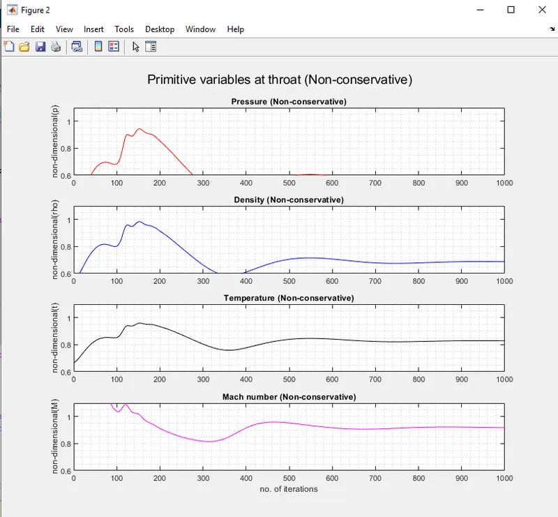
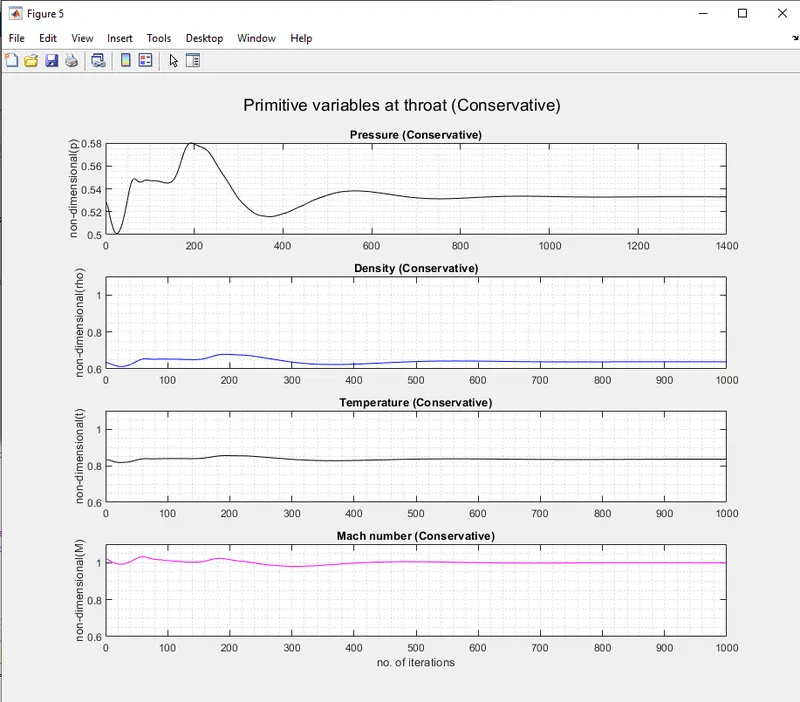
2. Time-wise variation of the primitive variables
a. Non-conservative:
b. Conservative:
4. Comparison of normalised mass flow rate distributions of both forms:
- Grid dependence test:
1. Non-Conservative:
n=31,
Density= 0.6387
temperature= 0.8365
Pressure= 0.5342
Mach number= 0.9994
n=61,
Density= 0.6377
temperature= 0.8354
Pressure= 0.5327
Mach number= 0.9998
2. Conservative:
n=31,
Density= 0.6524
temperature= 0.8411
Pressure= 0.5487
Mach number= 0.9780
n=61,
Density= 0.6390
temperature= 0.8357
Pressure= 0.5340
Mach number= 0.9978
3. Exact analytical values:
Density= 0.634
temperature= 0.833
Pressure= 0.528
Mach number= 1.000
- Conclusion/Results:
1. From the above results it is clear that the conservative solution does not vary in high amounts as compared to non-conservative solutions.
2. Computational time for conservative is less compared to the non-conservative solution.
3. From the grid independence test for the coarser nodes the non-conservative form gives accurate results and when the grid size is decreased with higher number of nodes, the conservtive solution gives better accurate results .
4. For the conservative form the solution do not blow up where as in the non-conservative form if the time step is not properly taken based on corants stability criteria the solution blows up.