Week 7: Shock tube simulation project

Aim

• Setup a transient shock tube simulation
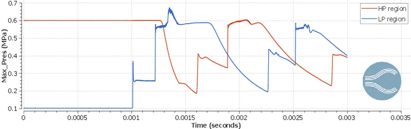
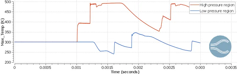
• Plot the pressure and temperature history in the entire domain - Explain the result
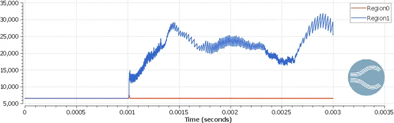
• Plot the cell count as a function of time - Explain the result

Shock Tubes

The shock tube is an instrument used to replicate and direct blast waves at a sensor or a model in order to simulate actual explosions and their effects, usually on a smaller scale. Shock tubes (and related impulse facilities such as shock tunnels, expansion tubes, and expansion tunnels) can also be used to study aerodynamic flow under a wide range of temperatures and pressures that are difficult to obtain in other types of testing facilities. Shock tubes are also used to investigate compressible flow phenomena and gas phase combustion reactions. More recently, shock tubes have been used in biomedical research to study how biological specimens are affected by blast waves.

A shock wave inside a shock tube may be generated by a small explosion (blast-driven) or by the buildup of high pressures which cause diaphragm(s) to burst and a shock wave to propagate down the shock tube (compressed-gas driven).

Geometry

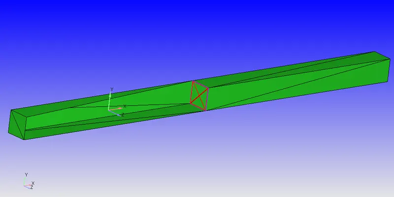
• Checked for errors
• Detected some manifold edges
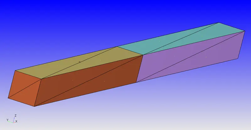
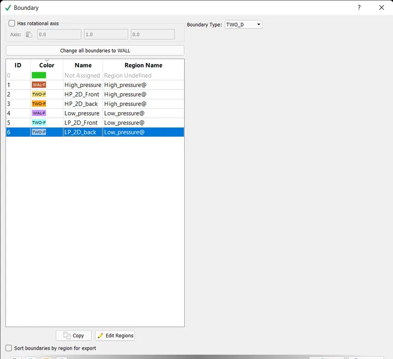
• Deleted the triangles present in between the two cuboids(In between the high pressure region and low pressure region)
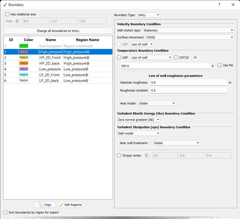
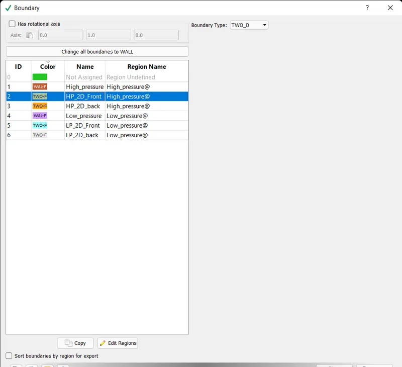
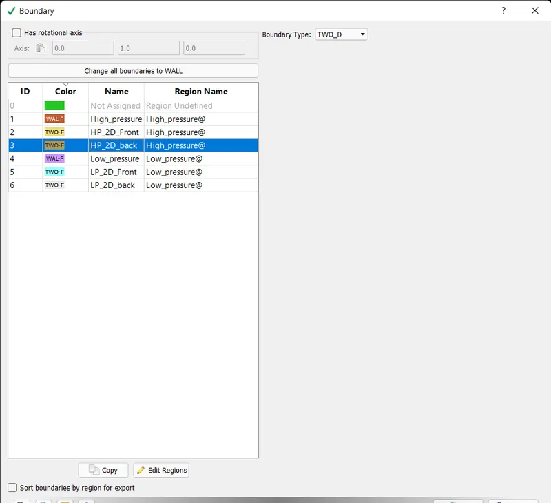
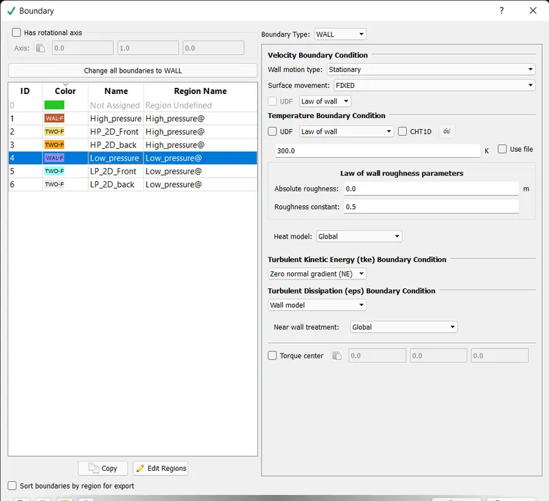
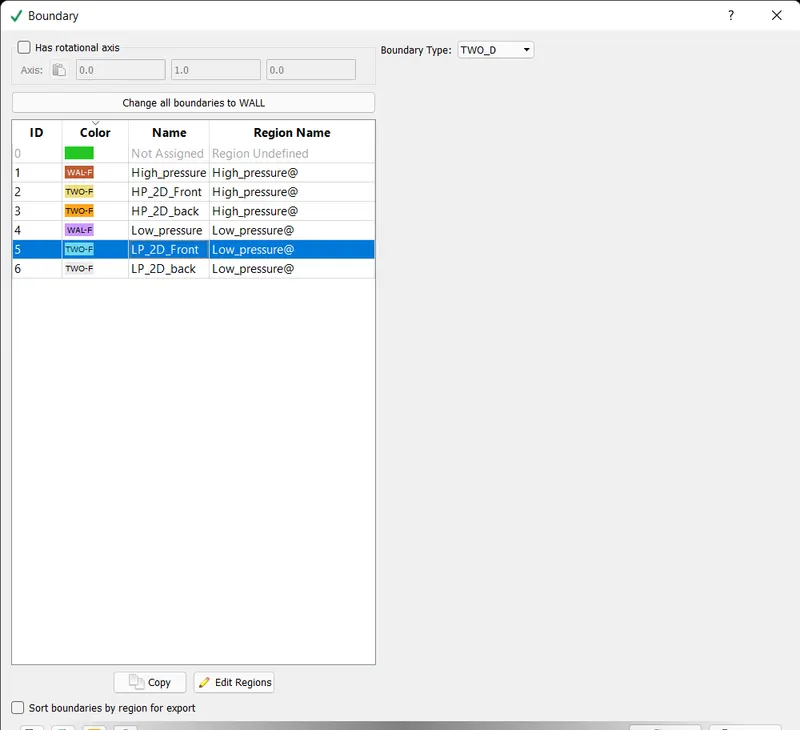
• Then Boundaries were flagged accordingly

Setup

• Time based simulation
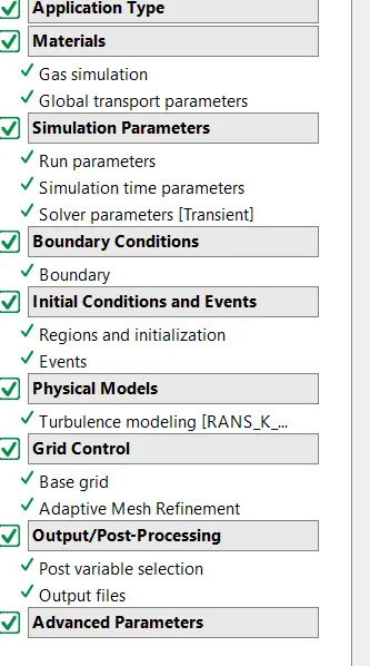
• In run parametres transient simulation is selected and Inernal energy solver is selected for energy solver
• Simulation is run from 0 to 0.003 with initial and minimum time steps being 1e-7 and the maximum time step being 1
• Pressure based simulation is selected
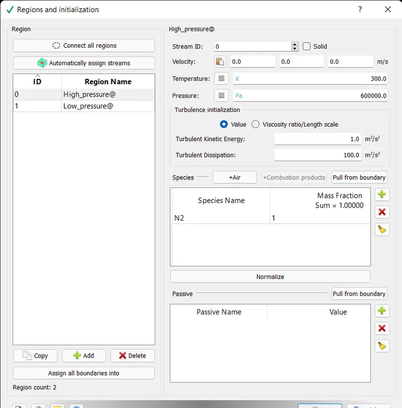
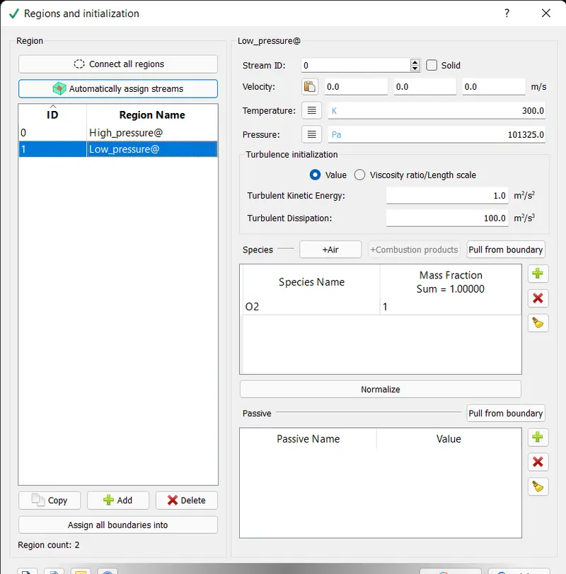
• Two region were defined with difference in its pressure values. The high pressure region contains a pressure of 6 bar and the low pressure region contain atmospheric pressure
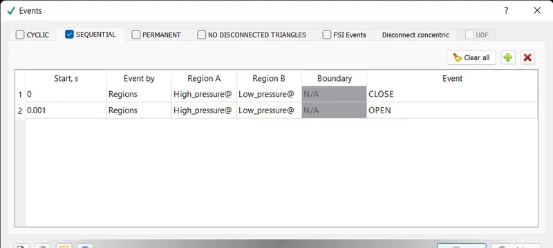
• Events were added to control the interaction so as to replace the diaphragm from the real case scenario
• Under physical models k-epsilon model were selected
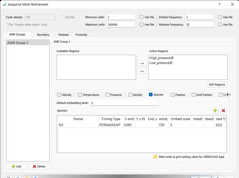
• Under grid control, Adaptive mesh refinement is added to enhance the visibility of the wave
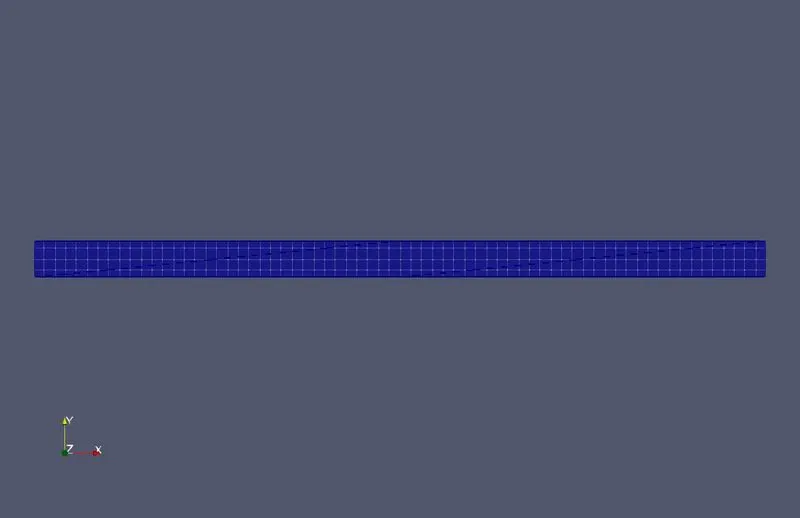
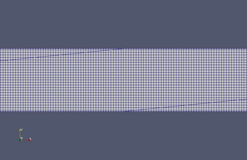
• The mesh size being 0.0004 m and Amr is set on species and Nitrogen is selected. The sub grid size being 0.001 with 3 embed layers (permenent)

Outputs

Mesh

AMR mesh animation

Plots

cells

Pressure contour

Pressure contour animation

Pressure plot along shock tube

Temperature contour

Temperature contour animation

Temperature plot along the shock tube

Velocity contour

Velocity contour animation

Velocity plot along shock tube

Observations

• From 0.001 seconds the cell count gets increased due to AMR. AMR succesfully captures the wave with fine cells.
• After 0.001 seconds the diaphragm bursts and a shock wave is developed
• The shock wave propagates through the shock tube back fourth
• When the pressure contour is observed it was seen that the pressure is higher at the bck side of wave propagation and pressure is lower at the front
• Due to compression the temperature is also more where the compression of gases is higher
• Shock propogates through the tube at higher velocity
• The gases move to both side right after the shock wave is created
• Velocity is higher to the right at first and when it got reflected due to different directions of gasses the movement suddenly stops

Conclusions

• Transient simulation to capture shock propagation was done
• Plotted temperature and pressure with time
• Cell counts were also plotted to analyse the effect of AMR