Week 7: Shock tube simulation project

SHOCK TUBE SIMULATION PROJECT

AIM: To run Transient Flow simulation in a Shock Tube using converge CFD.

OBJECTIVE

• Setup a transient shock tube simulation
• Plot the pressure and temperature history in the entire domain - Explain the result
• Plot the cell count as a function of time - Explain the result
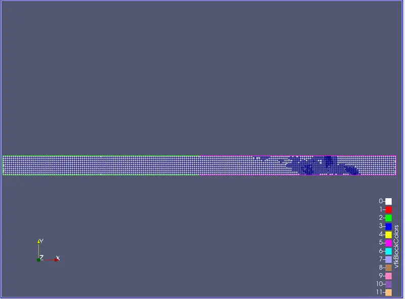
• It is expected to show the mesh generation using ParaView.

THEORY

The report contains a detailed description of the Shock tube Simulation problem using converge CFD software, solving it using CYGWIN, and post-processing the result using ParaView. This Case Study contains a rectangular duct that has two sections along with a diaphragm in between. A high-pressure reservoir is connected to the low-pressure section

A shock tube is a device for studying shock waves. Prior to starting an experiment, a diaphragm inside the tube blocks any flow. we can increase the pressure on one side, such as with a compressor, and then

start the flow by rupturing the diaphragm. The gas expands down the other half of the tube.

.

SIMULATION AND SOLUTION

Geometry

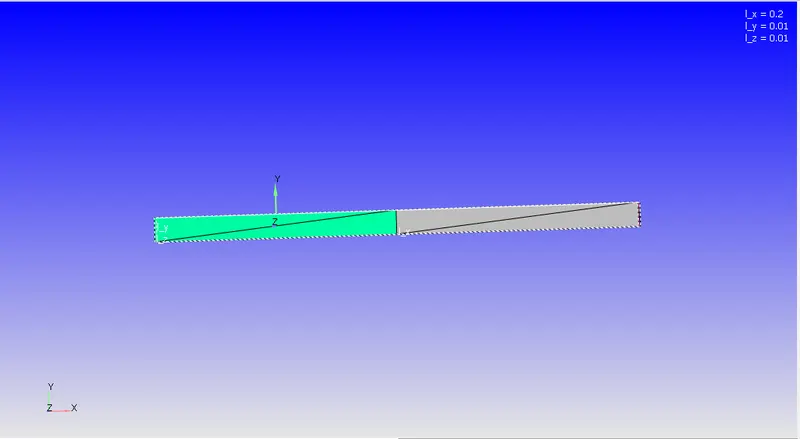
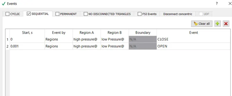
Using the given geometry we create 2 regions, which are the low-pressure region and the high-pressure region. By creating a diaphragm using events (time difference) we observe the results in the shock tube.

Setup:

Application Type	Time-based
MATERIALS:
1. Gas simulation	Standard
2. Global Transport Parameters	Standard
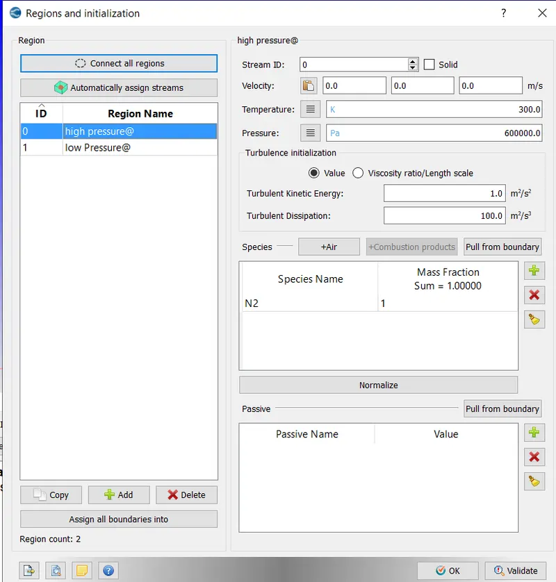
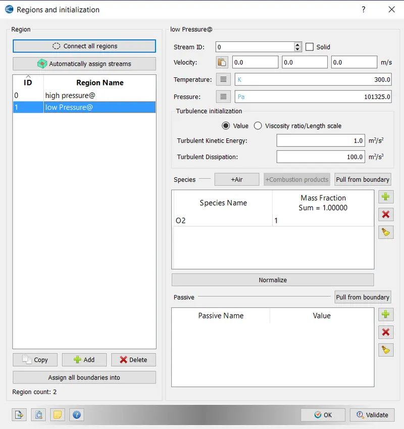
4. Species	1. fluid: O2 and N2
SOLUTION PARAMETERS
1. Run Parameters	Transient >Full hydrodynamic>Compressible
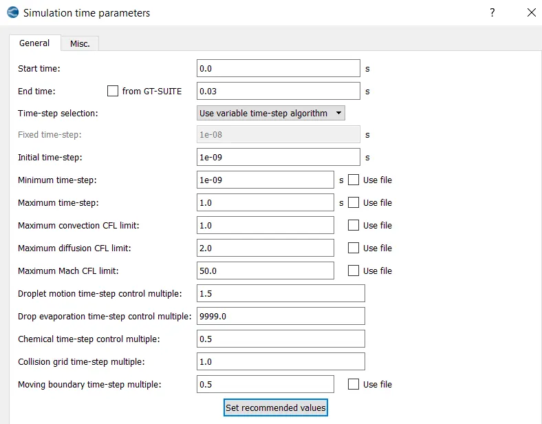
2. Simulation time parameters
3. Solver parameters	Navis-stokes solver scheme: PICO Navis-stokes solver type: density-based
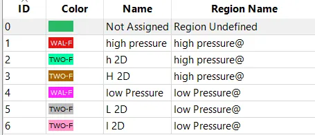
BOUNDARY CONDITIONS
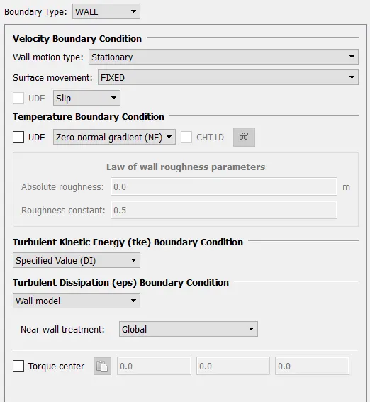
1. High pressure wall
2. High-pressure 2D front and Back	2D wall
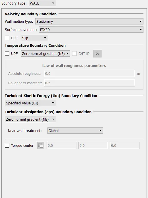
3. Low-pressure wall
4. Low-pressure 2D front and back wall	2D wall
INITIAL CONDITIONS AND EVENTS
1. Regions and initialization
2. EVENTS
PHYSICAL MODELS
1 Turbulence modeling	RNG- k-epsilon
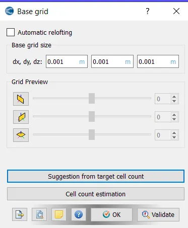
GRID CONTROL
1. Base mesh
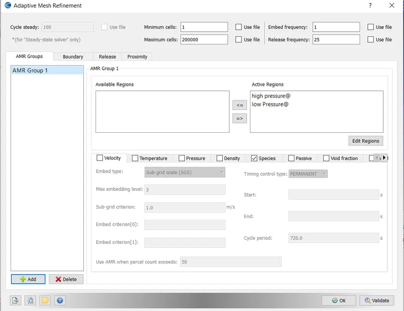
2. Adaptive meshing
OUTPUT/POST-PROCESSING
1. Post variable selection	Standard
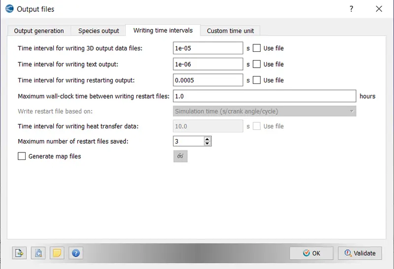
2. Output files:

Then Export the Files

Then continuing the setup in Cygwin :

• leading to the folder where the exported files are saved
• Then using mpiexec.exe -n 2 converge.exe restricted to simulate the setup
• After the output is generated, we lead the Cygwin to the output folder, and by copying the post_convert folder and
• Using mpiexec.exe -n 2 post_convert.exe and converting these files for processable output in ParaView.

Solution

Mesh

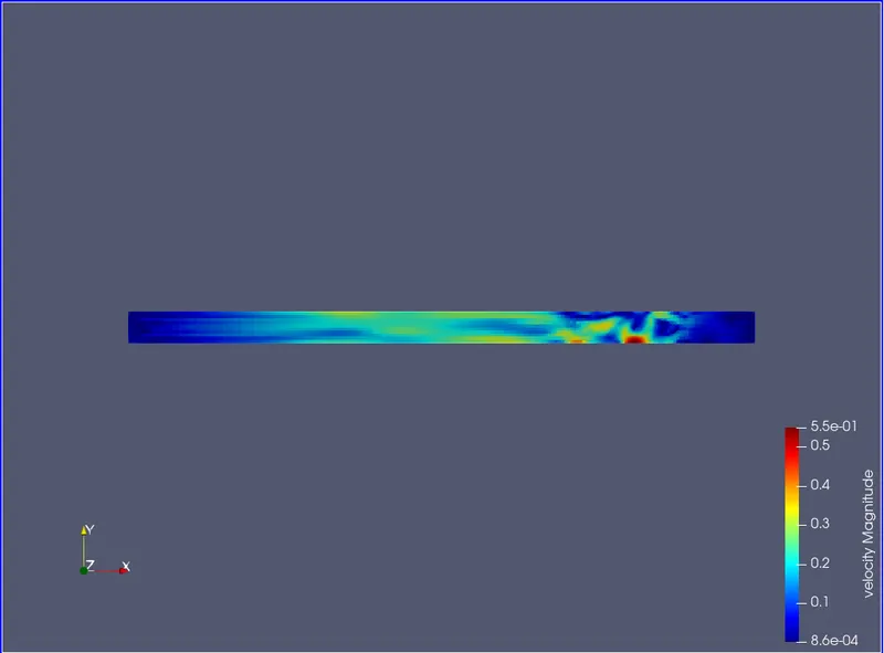
Velocity counter

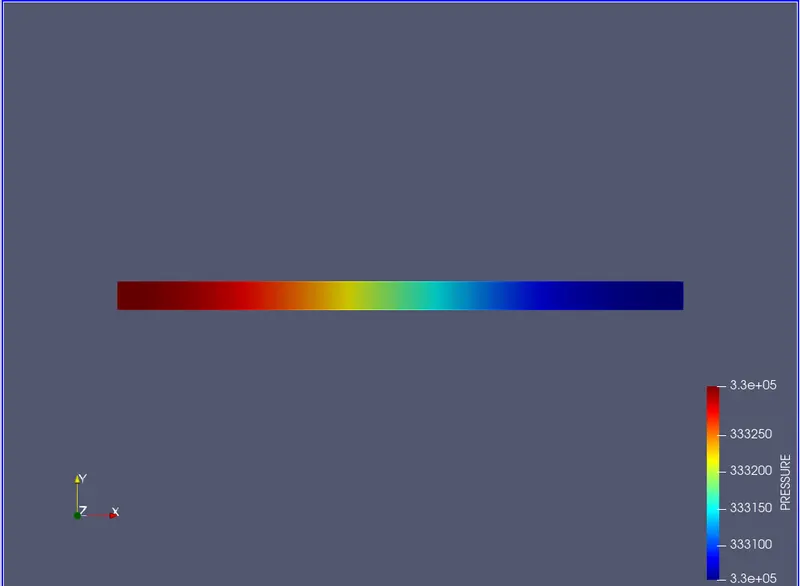
Pressure counter

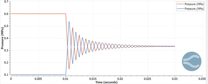
Pressure plot:

Pressure at thermo_region0.out and thermo_region1.out

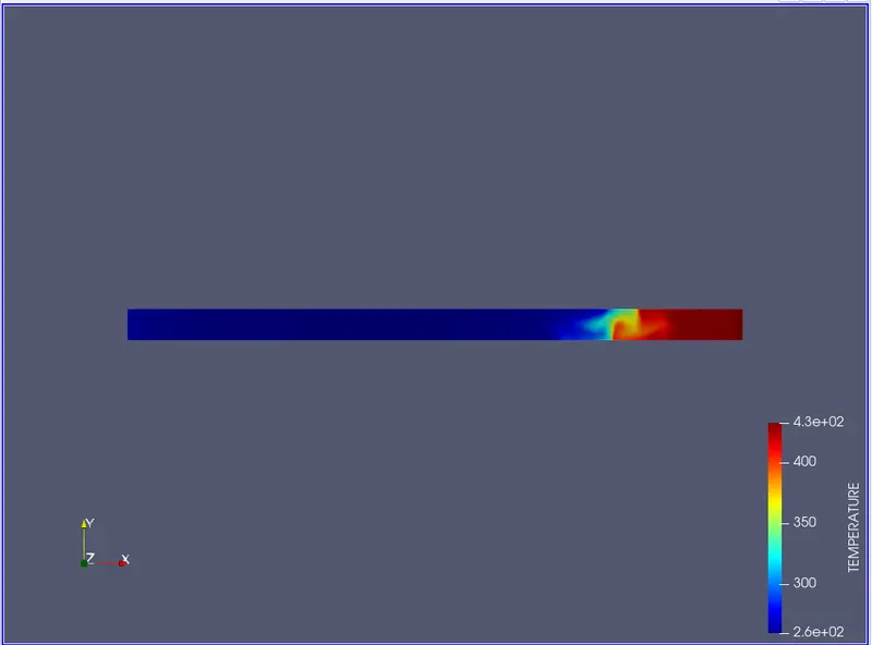
Temperature counter

Temperature plot

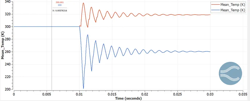
The temperature at thermo_region0.out and thermo_region1.out

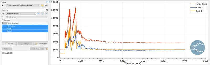
Cell count

CONCLUSION

• High-Pressure N2 gas compresses the low-pressure O2 then after some compression a recirculation takes places and the low-pressure gas passes the N2.
• From this problem, we can understand the compressibility of gas and study the flow.
• Due to adaptive mesh refinement, the cell count is varying all the time when the expansion and contraction are taking place inside the shock tube.
• From the pressure plot, it can be concluded that after some time both the species will have common pressure as one pressure is increasing and the other is decreasing wrt time.
• The temperatures first fluctuate then will attend the equilibrium position after some time.